1. Introduction
The dynamically high-quality response of a controller to the saturation of manipulated variables is an important task in controller design. Since such constraints represent non-linearities, the closed control loop is a non-linear system, even if the controlled system without actuator can be described as a linear, time-invariant system, which is assumed below. In order to avoid stability problems caused by the limitations of the manipulated variables, numerous so-called anti-windup methods are already known
| [1] | Hippe, P. Windup in Control. London: Springer; 2010. https://doi.org/10.1007/1-84628-323-X |
| [2] | Adamy, J. Nonlinear Systems and Controls. Berlin, Heidelberg: Springer Vieweg; 2022. https://doi.org/10.1007/978-3-662-65633-4 |
| [3] | Tarbouriech, S., Garcia, G., Goes da Silva Jr., J. M., Queinnec, I. Stability and Stabilization of Linear Systems with Saturating Actuators. London: Springer; 2011. https://doi.org/10.1007/978-0-85729-941-3 |
[1-3]
. For this purpose, the Popov criterion, the circle criterion, the direct method of Lyapunov or the Kalman-Yakubovich-Popov equations
| [2] | Adamy, J. Nonlinear Systems and Controls. Berlin, Heidelberg: Springer Vieweg; 2022. https://doi.org/10.1007/978-3-662-65633-4 |
| [3] | Tarbouriech, S., Garcia, G., Goes da Silva Jr., J. M., Queinnec, I. Stability and Stabilization of Linear Systems with Saturating Actuators. London: Springer; 2011. https://doi.org/10.1007/978-0-85729-941-3 |
| [4] | Vidyasagar, M. Nonlinear Systems Analysis. 2nd edition. Philadelphia: SIAM; 2002 (unabridged republication). https://doi.org/10.1137/1.9780898719185 |
[2-4]
are often used for stability considerations. In more recent research studies, so-called linear matrix inequalities (LMI) are also used as an alternative for stability studies. However, they often only provide numerical results
| [5] | Lerch, S., Dehnert, R., Damaszek, M., Tibken, B. Anti Windup PID Control of Discrete Systems Subject to Actuator Magnitude and Rate Saturation: An Iterative LMI Approach. Proceedings of the 25th International Conference on System Theory, Control and Computing (ICSTCC). Iasi, Romania, 2021, pp. 413–418. https://doi.org/10.1109/ICSTCC52150.2021.9607157 |
[5]
. Other current research work is concerned with the application of the basic principles of anti-windup measures to special controllers such as PI-lead controllers
| [6] | Chen, Y., Yang, M., Liu, K., Long, J., Xu, D., Blaabjerg, F. Reversed Structure Based PI-Lead Controller Antiwindup Design and Self-Commissioning Strategy for Servo Drive Systems. IEEE Transactions on Industrial Electronics. 2022, 69 (7), pp. 6586–6599. https://doi.org/10.1109/TIE.2021.3097602 |
[6]
or with switching strategies between different anti-windup measures
. In addition, the use of an
Additional Dynamic Element (ADE) is proposed, with which the stabilization in the limiting case succeeds for any controller stabilizing the unconstrained system
. However, even there a controller must be effective at least at one instance for which the stability in the limiting case can be proven – e.g. with the help of one of the methods listed above.
Stability analysis is especially challenging when the controller contains integral-action components to ensure steady-state accuracy. This is because the controller integral-action components are usually assigned to the controlled system during modeling, which results in an unstable or critically stable system. For this purpose, no positive definite matrices can be found for this, as required or at least aimed for in the Lyapunov theory and in the Kalman-Yakubovich-Popov equations to ensure stability. In
, this problem is overcome by completely avoiding controller integral-action components and instead attempting to ensure steady-state accuracy with the aid of disturbance observers. But this is not always possible when the system parameters are not exactly known. The method of reference variable correction in combination with a special PI-state controller design, as explained for example in
| [8] | Nuss, U. Stabilitätsverhalten von zweistufig entworfenen zeitdiskreten PI-Zustandsreglern bei Stellgrößenbegrenzungen [Stability properties of two-stage designed discrete-time PI state controllers considering the limitation of input variables]. at – Automatisierungstechnik. 2017, 65 (10), pp. 705 – 717. https://doi.org/10.1515/auto-2016-0136 (in German) |
| [9] | Nuss, U. Zeitdiskrete Regelung [Discrete-time control]. Berlin, Offenbach: VDE; 2020 (in German) |
[8, 9]
for discrete-time systems, provides a help in this respect. However, the stability proof described there has been greatly simplified in the meantime. Furthermore, by means of the above-mentioned procedure, it was also possible to perform the stability verification for such systems in a general way and thus greatly reduce the synthesis effort where the manipulated variables act on the system with dead time.
Due to the significant progress in stability verification for control loops with saturation of the manipulated variables, these new findings are presented in this article. The controlled system and the controller are modeled in state space. In section 2, as an introduction, the methodology of reference variable correction is first briefly explained for continuous-time systems and then the transfer to discrete-time systems is shown. Subsequently, section 3 describes special controller synthesis equations that generate a PI-state controller from an already known P-state controller in a simple way. In addition, both methods are combined in section 3 in order to establish the principles for a Lyapunov-based controller design for systems with an integral-action controller component, taking manipulated variable constraints into account. Using Lyapunov functions, the proof of stability is then provided in section 4. The measures mentioned are carried out for both continuous-time and discrete-time systems. In section 5, the method presented is extended to discrete-time systems with dead time behavior of the actuators. To illustrate the methods described, section 6 deals with an example from the field of electrical drives. A summary concludes the article.
2. Reference Variable Correction in Case of Manipulated Variable Saturation
2.1. State Equations of the Controlled System
The vectorial state differential equation of the controlled system,

,
(1)serves as the starting point for the following considerations
| [2] | Adamy, J. Nonlinear Systems and Controls. Berlin, Heidelberg: Springer Vieweg; 2022. https://doi.org/10.1007/978-3-662-65633-4 |
| [10] | Aström, K., Wittenmark, B. Computer-Controlled Systems. 2nd edition. Englewood Cliffs: Prentice-Hall; 1990 |
[2, 10]
. Here

denotes the

-dimensional state vector,

the

-dimensional manipulated variable vector,

the

-dimensional dynamics matrix and

the (

)-di mensional control input matrix. Disturbance variables are not considered without any generality restriction. Eq. (
1) is supplemented by the output equation
 (2)
(2)using the

-dimensional vector

of the control quantities and the (

)-dimensional output matrix

. The possibility of the manipulated variables affecting directly the control quantities is disregarded.
The differential or difference equations of the controller integrators are also included in the system description. In this respect, it is assumed below that there are as many controller integrators as controlled variables and as many reference variables as controlled variables. If the output variables of the controller integrators are summarized in the vector

and the reference variables in the vector

, then the vectorial differential equation of the controller integrators is as follows, provided they operate continuously in time,

.
(3)If the controlled system is described in discrete time, the controller design is based on the controlled system state difference equation
| [9] | Nuss, U. Zeitdiskrete Regelung [Discrete-time control]. Berlin, Offenbach: VDE; 2020 (in German) |
| [10] | Aström, K., Wittenmark, B. Computer-Controlled Systems. 2nd edition. Englewood Cliffs: Prentice-Hall; 1990 |
[9, 10]
 (4)
(4)instead of Eq. (
1). The indices

and

(

) indicate the sampling time instants

respectively

of the state variables and the time instants at which the manipulated variables take effect.

is the (

) -dimensional transition matrix for which
 (5)
(5)applies
| [9] | Nuss, U. Zeitdiskrete Regelung [Discrete-time control]. Berlin, Offenbach: VDE; 2020 (in German) |
| [10] | Aström, K., Wittenmark, B. Computer-Controlled Systems. 2nd edition. Englewood Cliffs: Prentice-Hall; 1990 |
[9, 10]
, while

is the discrete-time control input matrix with
| [9] | Nuss, U. Zeitdiskrete Regelung [Discrete-time control]. Berlin, Offenbach: VDE; 2020 (in German) |
| [10] | Aström, K., Wittenmark, B. Computer-Controlled Systems. 2nd edition. Englewood Cliffs: Prentice-Hall; 1990 |
[9, 10]

.
(6)
is the sampling time. The output equation is in the discrete-time case

.
(7)The vectorial difference equation of the controller integrators is as follows
| [9] | Nuss, U. Zeitdiskrete Regelung [Discrete-time control]. Berlin, Offenbach: VDE; 2020 (in German) |
| [10] | Aström, K., Wittenmark, B. Computer-Controlled Systems. 2nd edition. Englewood Cliffs: Prentice-Hall; 1990 |
[9, 10]

.
(8)2.2. Calculating the Corrected Reference Variables
The reference variable correction method for manipulated variable saturation
| [8] | Nuss, U. Stabilitätsverhalten von zweistufig entworfenen zeitdiskreten PI-Zustandsreglern bei Stellgrößenbegrenzungen [Stability properties of two-stage designed discrete-time PI state controllers considering the limitation of input variables]. at – Automatisierungstechnik. 2017, 65 (10), pp. 705 – 717. https://doi.org/10.1515/auto-2016-0136 (in German) |
| [9] | Nuss, U. Zeitdiskrete Regelung [Discrete-time control]. Berlin, Offenbach: VDE; 2020 (in German) |
[8, 9]
is based on the assumption that a manipulated variable saturation becomes effective because the setpoint change is too large. If this is the case, the maximum value by which the reference variable may be changed without the manipulated variable constraints becoming effective is calculated. The vector of reference variables corrected in this way is referred to below as

. To determine the value of
in the limiting case, the control law is specified firstly for the unlimited case and then again for the case of an active manipulated variable limitation. If the matrix of the feedback coefficients of the system state variables to the manipulated variable vector is denoted by

, the matrix of the feedback coefficients of the output variables of the controller integral-action components to the manipulated variable vector by

and the matrix of the amplification factors for the reference variables, the so-called pre-filter matrix, by

, then the control law in the unlimited case is as follows

.
(9)Thereby, the index
in brackets in Eq. (
9) only applies to the discrete-time case.
If a manipulated variable saturation now occurs, then instead of the manipulated variable vector
requested by the controller, only a manipulated variable vector modified by the saturation can act on the system. If this is designated as

, the control law
 (10)
(10)is obtained, which can be derived from Eq. (
9), if the possibly constrained manipulated variable vector

is used instead of

and the corrected reference variable vector

is used instead of

. The two relationships (
9) and (
10) can now be interpreted in such a way that they apply at the same time. Eq. (
9) generates the manipulated variable vector requested by the controller, while Eq. (
10) describes with which corrected reference variable vector the realizable manipulated variable vector
can be generated. If both equations are subtracted from each other and the resulting difference is solved for
, the result is as follows

.
(11)It specifies how
must be modified in order to obtain a realizable reference variable vector. The corrected reference variables are then fed to the setpoint inputs of the controller integrators. This means that instead of Eq. (
3), the following applies for continuous-time control

,
(12)whereas for discrete-time control, instead of Eq. (
8),
 (13)
(13)must be implemented. Thus, Eqs. (
9), (
11) and (
12) or respectively (
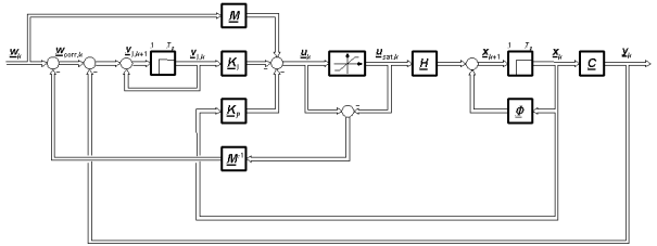
13) describe the equations of the controller. The corresponding block diagram is shown in
Figure 1 for the case of discrete-time control, including the discrete-time modeled controlled system. Finally, it should be noted that methods that also calculate corrected reference variables and use the difference between unlimited and limited manipulated variables are sometimes referred to as reverse-correction method
or back-calculation (and tracking) strategy
| [5] | Lerch, S., Dehnert, R., Damaszek, M., Tibken, B. Anti Windup PID Control of Discrete Systems Subject to Actuator Magnitude and Rate Saturation: An Iterative LMI Approach. Proceedings of the 25th International Conference on System Theory, Control and Computing (ICSTCC). Iasi, Romania, 2021, pp. 413–418. https://doi.org/10.1109/ICSTCC52150.2021.9607157 |
| [6] | Chen, Y., Yang, M., Liu, K., Long, J., Xu, D., Blaabjerg, F. Reversed Structure Based PI-Lead Controller Antiwindup Design and Self-Commissioning Strategy for Servo Drive Systems. IEEE Transactions on Industrial Electronics. 2022, 69 (7), pp. 6586–6599. https://doi.org/10.1109/TIE.2021.3097602 |
| [12] | March, P., Turner, C.. Anti-Windup Compensator Designs for Nonsalient Permanent-Magnet Synchronous Motor Speed Regulators. IEEE Transactions on Industry Applications. 2009, 45 (5), pp. 1598–1609. https://doi.org/10.1109/tia.2009.2027157 |
[5, 6, 12]
.
3. Relationship Between the Controller Coefficients of a PI-state Controller and a P-state Controller
In the study, it was shown how the coefficients of a discrete-time PI-state controller can be determined in a very simple way from an already calculated discrete-time P-state controller, provided that the same command response is to apply in both cases
| [9] | Nuss, U. Zeitdiskrete Regelung [Discrete-time control]. Berlin, Offenbach: VDE; 2020 (in German) |
| [13] | Nuss, U. Ein einfacher Zustandsreglerentwurf im Zuge der Erweiterung der Systemstruktur um Reglerintegratoren und Rechentotzeiten [A simple state space controller design in the context of expanding the control structure by integrators and calculation dead time]. at – Automatisierungstechnik. 2016, 64 (1), pp. 29–40. https://doi.org/10.1515/auto-2015-0058 (in German) |
[9, 13]
. The corresponding relationships for continuous-time state controllers were presented in
| [14] | Nuss, U. Regelungstechnik einfach verpackt [control theory simply presented]. forschung im fokus. Offenburg: University of Applied Science Offenburg. 2016, pp. 19 – 22. (in German) |
[14]
– and for single-input single-output systems also in
. With the designation

for the already known P-state controller, the following results for continuous-time controllers

,
(14)
,
(15)
,
(16)and for discrete-time systems

,
(17)
,
(18)
.
(19)With continuous-time control,

describes a diagonal matrix in which the main diagonal contains those control eigenvalues that have been added to the eigenvalues which result from the controlled system without controller integrators.

is the corresponding diagonal matrix for discrete-time systems. It should be emphasized in both cases that the control eigenvalues generated by
of the non-actuator-saturated P-state-controlled system are not changed by applying Eqs. (
9) and (
14) to (
16) or (
17) to (
19). It should also be noted that Eqs. (
14) to (
16) or (
17) to (
19) lead to
control eigenvalues that cannot be controlled via
(see section 4). Finally, it should be noted that the calculation rules (
16) and (
19) for the pre-filter matrix
are the same as the corresponding calculation rules for pure P-state controllers.
Figure 1. Block diagram of discrete-time PI-state control with reference variable correction in the case of manipulated variable saturation
If we now substitute Eq. (
9) into Eq. (
11) and the result for continuous-time control into Eq. (
12), we obtain, taking into account Eq. (
15),

.
(20)If this relationship is combined with the controlled system state differential equation (
1), but with
instead of
, to form an overall system, the following results
 (21)
(21)with

,
(22)
,
(23)
.
(24)In the case of discrete-time systems, by inserting Eq. (
9) into Eq. (
11) and inserting the resulting intermediate result into Eq. (
13) and taking Eq. (
18) into account, the following is obtained
 (25)
(25)The combination of this relationship with Eq. (
4), again with
instead of
, to form an overall system, taking into account Eq. (
22), gives the result
 (26)
(26)with

,
(27)
.
(28)It can now be seen that both the dynamic matrix

and the transition matrix

are lower block triangular matrices. Their eigenvalues are identical in their entirety with the eigenvalues of the matrix blocks on the main block diagonal. The eigenvalues of
are therefore composed of the eigenvalues of
and the control eigenvalues on the main diagonal of
caused by the controller integrators. For discrete-time systems, the eigenvalues of the transition matrix
are composed of the eigenvalues of
and the elements on the main diagonal of
, i.e. the control eigenvalues caused by the discrete-time controller integrators.
As the eigenvalues of
and
can be assumed to be stable, the dynamic matrix
and the transition matrix
each describe a stable system, provided the associated controlled system is stable. This is remarkable, especially as the controller integrators included in the model – considered on their own – show critically stable behavior. The reference variable correction according to Eq. (
11), in conjunction with the controller equations (
14) to (
16) respectively (
17) to (
19), has thus succeeded in forming a stable system from a critically stable system – assuming a stable controlled system but an unknown controller matrix
. Exactly this is extremely advantageous for the applicability of Lyapunov's direct method in stability analysis and controller synthesis for linear systems with manipulated variable limits (see section 4).
4. Controller Synthesis and Stability Verification
The stability analysis of PI-state control with manipulated variable saturation described below is based both on controllability considerations and on Lyapunov's direct method. In combination, both methods are also suitable for controller synthesis. Initially, however, the considerations focus on the stability analysis. In a first step, the system description according to Eq. (
21) respectively (
26) is transformed. The extended state vector

is mapped to the state vector

for continuous-time control using the transformation rules
 (29)
(29)
.
(30)Deriving Eq. (
29) with respect to time, replacing

by the right-hand side of Eq. (
21) and finally replacing
by Eq. (
29) solved for
then leads to the transformed differential state equation
 (31)
(31)with
 (32)
(32)and

.
(33)If in

and

the Eqs. (
14) to (
16) are taken into account, then after a few reforming steps the block diagonal matrix
 (34)
(34)arises and for
the result
 (35)
(35)is obtained. This shows that the lower
transformed state variables cannot be controlled from
, neither directly because of the zero matrix in
, nor indirectly via the upper

state variables because of the zero matrix in the lower block row of
. This means that the control eigenvalues contained in
cannot be controlled via
. As these eigenvalues can be considered to be stable, the subsystem described by the lower block row in
and
is both stable and not controllable and therefore does not need to be considered further in the stability investigations.
If the control is discrete-time, comparable statements can be made. Thus, the application of the transformation

,
(36) (37)
(37)to Eq. (
26), taking into account Eqs. (
17) to (
19), leads to the transformed state difference equation
 (38)
(38)with

,
(39)
.
(40)This also results in a subsystem that cannot be controlled via

, which has the eigenvalues contained in
that can be assumed as stable. Due to its stability and non-control lability, this subsystem can also be disregarded in the further stability investigations.
The previous explanations have shown that in both continuous-time and discrete-time system description and control, only the transformed first subsystem needs to be considered further for stability analysis after the state transformation has been carried out. However, this is precisely the controlled system with its manipulated variable vector
as the input variable. It is therefore sufficient to find a stabilizing control law for the controlled system using a P-state controller with the feedback matrix
. The stability of the resulting PI-state control by means of Eqs. (
14) to (
16) respectively (
17) to (
19) is then automatically ensured on the basis of the above explanations. In order to achieve a comparable statement for discrete-time systems, a complex modal transformation of the extended controlled system was carried out in
| [8] | Nuss, U. Stabilitätsverhalten von zweistufig entworfenen zeitdiskreten PI-Zustandsreglern bei Stellgrößenbegrenzungen [Stability properties of two-stage designed discrete-time PI state controllers considering the limitation of input variables]. at – Automatisierungstechnik. 2017, 65 (10), pp. 705 – 717. https://doi.org/10.1515/auto-2016-0136 (in German) |
[8]
. However, the above considerations have considerably simplified the proof. Comparable considerations have not yet been made for continuous-time systems.
To find a P-state controller that also stabilizes with manipulated variable limits, the following Lyapunov function is used

.
(41)In this,

denotes the deviation of the state vector

from its stationary position, which is denoted below by

. The following therefore applies

.
(42)Furthermore, the (
)-dimensional matrix

contained in Eq. (
41) must be a positive definite matrix yet to be determined. This means that

holds for

and

only for

. If it is now possible to ensure that

constantly decreases for
and approaches the steady state, i.e.

, for

then the stability of the system under consideration is proven
| [2] | Adamy, J. Nonlinear Systems and Controls. Berlin, Heidelberg: Springer Vieweg; 2022. https://doi.org/10.1007/978-3-662-65633-4 |
| [3] | Tarbouriech, S., Garcia, G., Goes da Silva Jr., J. M., Queinnec, I. Stability and Stabilization of Linear Systems with Saturating Actuators. London: Springer; 2011. https://doi.org/10.1007/978-0-85729-941-3 |
| [4] | Vidyasagar, M. Nonlinear Systems Analysis. 2nd edition. Philadelphia: SIAM; 2002 (unabridged republication). https://doi.org/10.1137/1.9780898719185 |
[2-4]
.
In order to be able to evaluate whether

decreases with a continuous-time system description,
is derived with respect to time and then the sign of

is examined. This results in

.
(43)
itself is obtained from the controlled system state differential equation (
1) with
instead of
. Here,
is also divided into a stationary component

and the deviation
 (44)
(44)of it. With further consideration of

, the following follows from the controlled system state differential equation

.
However, since

must be the zero vector in the steady state and
according to Eq. (
1) is identical with

in the steady state,

holds. Overall, this gives the state differential equation
 (45)
(45)for the deviation of the controlled system state vector from its stationary position. This used in Eq. (
43) then leads to

.
(46)For
to decrease for

,
must be negative. To ensure this even with saturated manipulated variables, the expression

is considered separately from the expression

. Because the former expression depends quadratically on

, it is generally to be expected that
reaches values which, due to the limitation of

, lead to such a large amount of
that this term determines the sign of
. The matrix term

is therefore assigned a positive definite or at most a positive semi-definite matrix

respectively

by
 (47)
(47)or

.
(48)It holds that if the matrix product

respectively

is positive definite, the matrix
is also positive definite if the controlled system is stable, i.e. if
only has eigenvalues with a negative real part
. Due to the special choice of the right-hand side of Eq. (
47),
can be any
-column matrix without violating the positive semi-definiteness of
. Only if
is to be positive definite, the number of rows of
must be at least as large as the number of columns of
and, in addition,

must apply
| [16] | Zurmühl, R., Falk, S. Matrizen und ihre Anwendungen [Matrices and their applications]. 5th edition. Berlin, Heidelberg, New York, Tokyo: Springer; 1984. (in German) |
[16]
. Furthermore, it should be noted that Eqs. (
47) and (
48) are Lyapunov equations. How they can be solved in principle can be read, for example, in
.
If there is a solution for
in Eq. (
47) or (
48), then it can be enforced that the right-hand side of Eq. (
46) does not become positive, provided the controlled system is asymptotically stable or critically stable. To do this,

is set in the way
 (49)
(49)where

is a positive definite (

) -dimensional diagonal matrix with otherwise arbitrary diagonal elements and

is an arbitrary matrix of suitable dimension, provided that Eq. (
47) is used as the basis for
. When using Eq. (
48),

must be selected. The chosen approach based on Eq. (
47) is oriented towards the so-called Kalman-Yakubovich-Popov equations
| [2] | Adamy, J. Nonlinear Systems and Controls. Berlin, Heidelberg: Springer Vieweg; 2022. https://doi.org/10.1007/978-3-662-65633-4 |
| [3] | Tarbouriech, S., Garcia, G., Goes da Silva Jr., J. M., Queinnec, I. Stability and Stabilization of Linear Systems with Saturating Actuators. London: Springer; 2011. https://doi.org/10.1007/978-0-85729-941-3 |
| [4] | Vidyasagar, M. Nonlinear Systems Analysis. 2nd edition. Philadelphia: SIAM; 2002 (unabridged republication). https://doi.org/10.1137/1.9780898719185 |
[2-4]
, which generally results in more degrees of freedom than the more classical approach based on Eq. (
48) with
. However, it is often sufficient to work with
and the somewhat more simply structured formulas, using either Eq. (
47) or Eq. (
48) as a basis.
Eq. (
49) implies the controller matrix

.
(50)With this and Eqs. (
46), (
47) and (
49) we obtain


.
(51)If
is now chosen so that

is positive definite – for which the diagonal elements of
only have to be chosen sufficiently large – then

is a positive semi-definite matrix term
| [16] | Zurmühl, R., Falk, S. Matrizen und ihre Anwendungen [Matrices and their applications]. 5th edition. Berlin, Heidelberg, New York, Tokyo: Springer; 1984. (in German) |
[16]
due to

. Furthermore,

is also at least positive semi-definite. This ensures that
does not become positive. With

,
quadratic and positive definite and
positive definite in any case,
is then always negative for

and zero for

itself.
is negative definite in this case, while
is positive definite. Since these properties apply to the entire state space, the stability condition of Lyapunov's direct method is fulfilled and thus the system under consideration is stable
| [2] | Adamy, J. Nonlinear Systems and Controls. Berlin, Heidelberg: Springer Vieweg; 2022. https://doi.org/10.1007/978-3-662-65633-4 |
| [3] | Tarbouriech, S., Garcia, G., Goes da Silva Jr., J. M., Queinnec, I. Stability and Stabilization of Linear Systems with Saturating Actuators. London: Springer; 2011. https://doi.org/10.1007/978-0-85729-941-3 |
| [4] | Vidyasagar, M. Nonlinear Systems Analysis. 2nd edition. Philadelphia: SIAM; 2002 (unabridged republication). https://doi.org/10.1137/1.9780898719185 |
[2-4]
. The same applies if the considerations are based on Eq. (
48), which with
results in

.
(52)Both, Eqs. (
51) and (
52), also apply in particular when manipulated variable constraints take effect. In this case, the limitation causes the amount of a certain element of
to be smaller than specified by the controller. However, this can be modeled according to Eq. (
49) by a corresponding increase in the relevant diagonal element of
. However, since the diagonal elements of
can be chosen to be arbitrarily large as long as they are only positive and fulfill the condition

, this has no negative influence on the definiteness of

and thus on the stability conclusion.
It is particularly worth mentioning in this context that for the proof of stability described above, both matrices

and
must be positive definite if
is positive definite and
is negative definite. This is possible if the controlled system is stable. However, if the controller integrators had been included in the system model without splitting off the uncontrollable, stable subsystem as described above, then the simultaneous specification of
and
as positive definite matrices would not have been possible due to the then critically stable system.
If the description of the controlled system is available in discrete-time form, the difference
 (53)
(53)is formed. If it is negative definite,

decreases at each sampling step as long as

is not a zero vector. The aim is therefore to ensure that

is negative definite in the entire state space. For this purpose,

and
are replaced in Eq. (
53) according to the right-hand side of Eq. (
41), from which
 (54)
(54)follows. Furthermore, for

according to Eqs. (
4) and (
42), but with
instead of

, we obtain
 (55)
(55)In addition, Eq. (
4) leads to the following relationship for the steady state due to

and

:
From Eq. (
55) therefore arises

.
(56)If we now insert Eq. (
56) into Eq. (
54), we finally receive
 (57)
(57)If we proceed according to Lyapunov's direct method, we must first ensure that the first summand

is negative definite or at least negative semi-definite. This is ensured by
 (58)
(58)respectively
 (59)
(59)and by setting
as a matrix with at least as many rows as columns at maximum rank when applying Eq. (
58) and aiming for positive definiteness of

as in the continuous-time system description. If
only has stable eigenvalues, then the positive definiteness of
follows from the positive definiteness of
respectively
and thus also the positive definiteness of

according to Eq. (
41). If, on the other hand,
has stable and/or critically stable eigenvalues,
can be chosen to be positive definite, but
respectively
can then at best be positive semi-definite (see example from section 6).
In order for
to be negative (semi-)definite, the sum of all three summands must be negative (semi-)definite in addition to the first summand of Eq. (
57), which can now be represented in the form

respectively

. To achieve this, starting from the second summand, the control law
 (60)
(60)or the associated controller matrix
 (61)
(61)is applied – if applicable with
in the case of Eq. (
59). Eq. (
60), after insertion into Eq. (
57) and taking into account Eqs. (
58) and (
61) yields the result

.
(62)Using Eq. (
59) as a basis,
is then simply specified as the zero matrix and
is replaced by
. If
is now chosen so that the bracket expression

is positive definite, then the entire matrix term in the last row of Eq. (
62) is positive semi-definite due to

. Again, this can always be achieved with sufficiently large amounts

(

) of
. Furthermore, because the matrix term in the second last row of Eq. (
62) is at least positive semi-definite,
cannot become positive. With
, quadratic, positive definite specification of
and

, a stable discrete-time controlled system according to Eq. (
4) can therefore always be stabilized using the control law (
60) via a PI-state controller. This also applies in particular when manipulated variable constraints occur, because when limiting

(
), only the element
of
needs to be increased in thought until
corresponds to the relevant limiting value using Eq. (
60).
5. Discrete-time Systems with Dead Time for Manipulated Variable Determination
With discrete-time systems, it is often the case that the manipulated variables do not act on the system – not even approximately – from the instant at which the state variables from which the respective manipulated variables were determined are sampled. A dead time between the calculation of the manipulated variables and their becoming effective must therefore be taken into account when creating the model. In order to have defined and at the same time easily manageable correlations, a dead time is usually introduced that incorporates exactly one sampling interval
| [9] | Nuss, U. Zeitdiskrete Regelung [Discrete-time control]. Berlin, Offenbach: VDE; 2020 (in German) |
| [13] | Nuss, U. Ein einfacher Zustandsreglerentwurf im Zuge der Erweiterung der Systemstruktur um Reglerintegratoren und Rechentotzeiten [A simple state space controller design in the context of expanding the control structure by integrators and calculation dead time]. at – Automatisierungstechnik. 2016, 64 (1), pp. 29–40. https://doi.org/10.1515/auto-2015-0058 (in German) |
[9, 13]
. The calculated, if necessary limited manipulated variable vector
, which was determined on the basis of the state vector

, is then set to a newly introduced vector

, using the difference equation

.
(63)If

is now used instead of
as the manipulated variable vector acting on the controlled system, the dead time is taken into account in the model. If
and
are then combined to form the overall state vector
 (64)
(64)this results in the vectorial controlled system state difference equation
,
(65)using the extended transition matrix
 (66)
(66)and the extended discrete-time control input matrix

.
(67)For the output equation of the system with dead time, it is correspondingly obtained
 (68)
(68)with

.
(69)If it is now successful to establish a generally valid correlation between the stability behavior of the system extended by dead times and the dead-time-free system with and without manipulated variable constraints, then the effort for stability analysis and controller synthesis can be significantly reduced for systems with manipulated variable saturation and dead times in the manipulated variable paths.
For the difference equation (
65) of the controlled system with dead time, the same stability considerations can now be made as those based on the system state difference equation (
4). Analogous to Eq. (
57), the relationship
then occurs, where first for

and then for the remaining terms negative definiteness or negative semi-definiteness must be ensured. With the approaches

,
(71) (72)
(72)respectively

instead of

and at the same time

, this is achieved in the same way as previously described in section 4 for discrete-time systems without dead times in the manipulated variable paths. If you now specify

as a symmetrical matrix in block matrix notation

,
(73) as block diagonal matrix
 (74)
(74)and

in block matrix notation

,
(75)then it follows from Eq. (
71) by block-by-block writing, taking into account Eq. (
66)

,
(76)
,
(77)
.
(78)While Eq. (
76) represents the discrete-time Lyapunov equation of the dead time-free controlled system, Eqs. (
77) and (
78) directly yield the solutions

,
(79) (80)
(80)for the matrix blocks

and

of
. The specification of
therefore determines
. Because
is positive definite if
respectively
with stable transition matrix
is positive definite
and
as upper block triangular matrix with stable matrix
fulfills this condition, the positive definiteness of
no longer needs to be proven separately. If we also evaluate Eq. (
61) for
according to Eq. (
73) instead of
,
according to Eq. (
66) instead of
,

according to Eq. (
67) instead of
,
according to Eq. (
74) instead of
and
according to Eq. (
75) instead of
, then the following results with

instead of
, taking into account Eq. (
79):

.
(81)A comparison with Eq. (
61) shows that for
the controller matrix
of the system with dead time is associated with the controller matrix
of the system without dead time via the relationship

.
(82)In
| [13] | Nuss, U. Ein einfacher Zustandsreglerentwurf im Zuge der Erweiterung der Systemstruktur um Reglerintegratoren und Rechentotzeiten [A simple state space controller design in the context of expanding the control structure by integrators and calculation dead time]. at – Automatisierungstechnik. 2016, 64 (1), pp. 29–40. https://doi.org/10.1515/auto-2015-0058 (in German) |
[13]
, Eq. (
82) was already derived – without taking manipulated variable limits into account – for the problem that a controller matrix (here
) is requested for the system with dead time, which produces the same control behavior as the associated dead time-free system, only delayed by one sampling interval. Interestingly, this controller setting also fulfills the requirement for stability in the case of manipulated variable constraints, provided that the dead time-free system (with the controller matrix
) fulfills this requirement. Furthermore, when applying Eq. (
82), the pre-filter matrix ensuring stationary accuracy in the command behavior, which is denoted below as

to distinguish it from
from Eq. (
19), is identical to
, i.e. it holds

.
(83)To recognize this, the determination equation for
is first written according to Eq. (
19) with

instead of
,
instead of
,
instead of
and
instead of
. It reads

.
(84)In this context, taking into account Eqs. (
66) and (
67), it holds
 (85)
(85)as well as
 (86)
(86)The easiest way to verify the above relationship is to multiply

by

to obtain the unit matrix. If
is then multiplied from the left by
according to Eq. (
69) and from the right by
according to Eq. (
67), the following results

,
which just equals

. The renewed inversion and negation according to Eq. (
84) finally leads to the statement of Eq. (
83).
Finally, it should be noted that the stability statement made in this section also applies if the controlled system includes a dead time in the maniplated variable paths and is to be controlled with a PI-state controller. In this case, as described above, a P-state controller is first designed for the controlled system with dead time using Eqs. (
82) and (
83) (without controller integral-action component) and then

from Eq. (
82) is inserted as the controller matrix

in Eq. (
17). The extended system matrices

,

and

from Eqs. (
66), (
67) respectively (
69) can be used. The pre-filter matrix

can remain unchanged due to Eq. (
83) and the statements in section 3.
6. Example
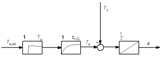
The following example from the field of electrical drives is intended to illustrate the methodology described above. It concerns the speed control system of a three-phase drive to be controlled. The associated model consists of the series connection of a dead time element and a P-T
1 element to simulate the subordinate closed current control loop as well as an integrator to model the mechanics (single-mass oscillator).
Figure 2 shows the continuous-time structure of the model. To concentrate on the essentials, the setpoint

respectively the actual value

of the electric torque are used directly as input and output variables of the subordinate current control loop instead of the corresponding torque-forming current (setpoint) components. The time constant of the closed current control loop is

. The dead time element comes from the modeling of the computing time of the signal processor used for control. The difference between the electric torque
and the load torque

results in the acceleration torque, which leads to the speed (angular velocity)

when integrated via the moment of inertia

.
Figure 2. Continuous-time block diagram of the exemplary controlled system.
A discrete-time PI-state controller is to be used as the speed controller. For this purpose, the system model must be discretized beforehand. Using the sampling time
and neglecting the load torque, the discrete-time state equations of the dead-time-free system are approximately as follows
| [8] | Nuss, U. Stabilitätsverhalten von zweistufig entworfenen zeitdiskreten PI-Zustandsreglern bei Stellgrößenbegrenzungen [Stability properties of two-stage designed discrete-time PI state controllers considering the limitation of input variables]. at – Automatisierungstechnik. 2017, 65 (10), pp. 705 – 717. https://doi.org/10.1515/auto-2016-0136 (in German) |
| [17] | Nuss, U. Hochdynamische Regelung elektrischer Antriebe [Highly dynamic control of electrical drives]. 2nd edition. Berlin, Offenbach: VDE; 2017. (in German) |
[8, 17]

,

,

,
if the state variable

is understood to be the actual torque value and the state variable

, which is also the controlled variable

, is understood to be the actual speed value. In contrast, the output variable of the dead time element from
Figure 2 serves as the manipulated variable

in the dead time-free system. For

, it holds

. For the relevant system matrices, this results in the values

,

,

.
As can easily be seen, the transition matrix
has an eigenvalue at

, which is why the controlled system is not asymptotically stable. It can therefore be assumed that
respectively
will not be a positive definite matrix term. The calculation of

according to Eq. (
58) or (
59) shows this immediately. Because with the symmetrical matrix
and the abbreviation

you get
Because of the zero element on the main diagonal,
respectively
can at best be positive semi-definite, and only if the secondary diagonal elements are zero. From this follows directly

.
Since it is sufficient for the example to carry out the controller calculation with
and thus use Eq. (
48) as a basis, it applies that

.
Finally, the condition
must be fulfilled so that
can be positive semi-definite. For the matrix
, it follows under the above conditions

.
It has positive definiteness for

and

. Furthermore, the positive semi-definiteness of
must also be fulfilled, which leads in the example to the condition
using

. In the next step, the P-state controller matrix
is calculated by means of Eq. (
61). Because
was selected, the result is

.
If, for example,

holds and

is chosen without restricting the generality, then

and

, for example, fulfill the above conditions. For
and
, it follows from this, but for general

,

,

.
If the controlled system model is then extended by the dead time element, Eq. (
82) immediately provides the extended controller matrix

.
Finally, if a controller integral-action component with the eigenvalue

assigned to it is added, it follows from Eqs. (
17) and (
18)

,

.
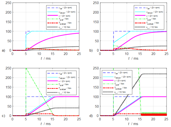
Figure 3 shows the transient response that is achieved. Here, a speed setpoint step from 0 to

is specified at time

with vanishing initial state variable values. The step height was intentionally chosen so large that the manipulated variable of the speed controller, i.e. the torque setpoint
, reaches the limit

at the start of the transient response. In addition to the uncorrected speed setpoint

, the actual speed value
and the unlimited torque setpoint
,
Figure 3 also shows the corrected speed setpoint

, the saturated torque setpoint

and the output variable

of the speed controller integrator. With regard to the latter, it should be noted that
Figure 3 is based on the fact that the control difference is first multiplied by

and only then integrated and fed to the manipulated variable determination with a positive sign. In addition to the aforementioned value
for the weighting factor,
Figure 3 also shows curves for other values of the weighting factor
in order to demonstrate its influence on the control quality. All diagrams are based on the moment of inertia

and the sampling time

.
As can be clearly seen in
Figure 3, the control loop dynamics continue to increase as the weighting factor
decreases. At

, however, there appears a clear torque ripple. But, at
, the previously mentioned sufficient stability condition is no longer fulfilled. Since this is only a sufficient condition, stable operation cannot be excluded, which is also shown in principle in
Figure 3d.
Figure 3. Transient response of the relevant variables of the speed control loop when a speed setpoint step is specified with a limited torque setpoint; a) r=10, b) r=5, c) r=0,5, d) r=0,05.