Many real-world phenomena such as nerve pulse transmission, fluid transport, and chemical kinetics are modeled using nonlinear partial differential equations with time-fractional derivatives. Among them, the time-fractional Burgers-Huxley equation plays a significant role due to its ability to capture both diffusion and reaction mechanisms with memory effects. Solving such equations in higher dimensions is highly challenging and calls for efficient analytical approaches. In this work we present a technique for handling the time-fractional Burgers-Huxley equation up to k-dimensions by employing Laplace transform based homotopy perturbation method (LT-HPM). The LT-HPM is adopted based on its advantage in dealing with nonlinear terms and simplify the solution process by converting fractional derivatives into more manageable expressions. Unlike other hybrid approaches, LT-HPM is less computational complex and provides rapid convergent series solutions without requiring any linearization or restrictive assumptions. To showcase the effectiveness of this approach, we solve a pair of examples: a 2-D case and a 3-D case. The obtained results confirm that LT-HPM is accurate and powerful in tackling complex nonlinear PDEs in higher dimensions.
| Published in | American Journal of Applied Mathematics (Volume 13, Issue 4) |
| DOI | 10.11648/j.ajam.20251304.12 |
| Page(s) | 245-255 |
| Creative Commons |
This is an Open Access article, distributed under the terms of the Creative Commons Attribution 4.0 International License (http://creativecommons.org/licenses/by/4.0/), which permits unrestricted use, distribution and reproduction in any medium or format, provided the original work is properly cited. |
| Copyright |
Copyright © The Author(s), 2025. Published by Science Publishing Group |
Time Fractional Burgers-Huxley Equation, Homotopy Perturbation Method, Laplace Transform
(x, y) | Exact Solutions | LTHPM Solutions | Absolute Errors |
|---|---|---|---|
(0.5, 0.5) | 0.6124335747 | 0.6123276002 | 1.0597e-004 |
(1.0, 1.0) | 0.7621140571 | 0.7620974978 | 1.6559e-005 |
(1.5, 1.5) | 0.8666142484 | 0.8666109783 | 3.2701e-006 |
(2.0, 2.0) | 0.9294637452 | 0.9294602148 | 3.5304e-006 |
(2.5, 2.5) | 0.9639321910 | 0.9639291906 | 3.0004e-006 |
(3.0, 3.0) | 0.9818852652 | 0.9818833425 | 1.9228e-006 |
(3.5, 3.5) | 0.9909855209 | 0.9909844454 | 1.0755e-006 |
(4.0, 4.0) | 0.9955348667 | 0.9955343028 | 5.6388e-007 |
(4.5, 4.5) | 0.9977933951 | 0.9977931086 | 2.8652e-007 |
(5.0, 5.0) | 0.9989107756 | 0.9989106322 | 1.4338e-007 |
(x, y) | Exact Solutions | LTHPM Solutions | Absolute Errors |
|---|---|---|---|
(0.5, 0.5) | 0.3213377612 | 0.3115477770 | 9.7900e-003 |
(1.0, 1.0) | 0.4624931076 | 0.4785665336 | 1.6073e-002 |
(1.5, 1.5) | 0.6433724822 | 0.6505187805 | 7.1463e-003 |
(2.0, 2.0) | 0.7924064045 | 0.7905803437 | 1.8261e-003 |
(2.5, 2.5) | 0.8883081188 | 0.8844777193 | 3.8304e-003 |
(3.0, 3.0) | 0.9424258906 | 0.9394963754 | 2.9295e-003 |
(3.5, 3.5) | 0.9709729155 | 0.9692236087 | 1.7493e-003 |
(4.0, 4.0) | 0.9855284143 | 0.9845846217 | 9.4379e-004 |
(4.5, 4.5) | 0.9928253260 | 0.9923392947 | 4.8603e-004 |
(5.0, 5.0) | 0.9964528080 | 0.9962080201 | 2.4479e-004 |
(x, y,) | Exact Solutions | LTHPM Solutions | Absolute Errors |
|---|---|---|---|
(0.5, 0.5, 0.5) | 0.2455838481 | 0.2450850131 | 4.9884e-004 |
(1.0, 1.0, 0.5) | 0.1647457980 | 0.1645164628 | 2.2934e-004 |
(1.5, 1.5, 0.5) | 0.1067702642 | 0.1066905939 | 7.9670e-005 |
(2.0, 2.0, 0.5) | 0.0675591813 | 0.0675466911 | 1.2490e-005 |
(2.5, 2.5, 0.5) | 0.0420772486 | 0.0420877279 | 1.0479e-005 |
(3.0, 3.0, 0.5) | 0.0259429019 | 0.0259573571 | 1.4455e-005 |
(3.5, 3.5, 0.5) | 0.0158942527 | 0.0159063917 | 1.2139e-005 |
(4.0, 4.0, 0.5) | 0.0096997752 | 0.0097084764 | 8.7012e-006 |
(4.5, 4.5, 0.5) | 0.0059052753 | 0.0059110688 | 5.7935e-006 |
(5.0, 5.0, 0.5) | 0.0035898933 | 0.0035936025 | 3.7093e-006 |
HPM | Homotopy Perturbation Method |
LT-HPM | Laplace Transform Homotopy Perturbation METHOD |
TFBH | Time Fractional Burgers-Huxley Equation |
VIM | Variational Iteration Method |
ADM | Adomian Decomposition Method |
PDEs | Partial Differential Equations |
ODEs | Ordinary Differential Equations |
2-D | 2 Dimensional |
3-D | 3 Dimensional |
| [1] | He, J. H. Homotopy perturbation technique. Computer Methods in Applied Mechanics and Engineering. 1999, 178, 257-262. |
| [2] | He, J. H. A coupling method of a homotopy technique and a perturbation technique for non-linear problems. International Journal of Non-Linear Mechanics. 2000, 35, 37-43. |
| [3] | He, J. H. Some applications of nonlinear fractional differential equations and their approximations. Bulletin of Science, Technology & Society. 1999, 15, 86-90. |
| [4] | He, J. H. Application of homotopy perturbation method to nonlinear wave equations. Chaos, Solitons and Fractals. 2005, 26, 695-700. |
| [5] | Hussain, A., Bano S., Khan L., Baleanu D., Nisar K. S. Lie symmetry analysis, explicit solutions and conservation laws of a two-dimensional Burgers-Huxley equation. Symmetry. 2020, 12(1). |
| [6] | Inc, M., Yusuf A., Baleanu D. Lie symmetry analysis and explicit solutions for the time fractional generalized Burgers-Huxley equation. Optical and Quantum Electronics. 2018, 50(94). |
| [7] | Kushner, A. G., Matviychuk R. I. Exact solutions of the Burgers-Huxley equation via dynamics. Journal of Geometry and Physics. 2020, 151(6). |
| [8] | Feng, Z., Tian, J., Zheng, S., Lu H. Travelling wave solution of the Burgers-Huxley equation. IMA Journal of Applied Mathematics. 2012, 77(3), 316-325. |
| [9] | Wazwaz, A. M., Travelling wave solutions of generalized forms of Burgers, Burgers-KDV and Burgers-Huxley equation. Applied Mathematics and Computation. 2005, 169(1), 639-656. |
| [10] | Zhang, X., Tial, Y., Qi, Y. Mathematical studies on generalized Burgers-Huxley equation and its singularly perturbed form: existence of traveling wave solutions. Nonlinear Dynamics. 2024, 113, 2625-2634. |
| [11] | Wang, X. Y., Zhu, Z., Lu, Y. K. Solitary wave solutions of the generalized Burgers-Huxley equation. Journal of Physics A: Mathematical and General. 1990, 23(3), 271-274. |
| [12] | Kamboj, D., Sharma, M. D. Singularly perturbed Burgers-Huxley equation: analytical solution through iteration. International Journal of Engineering Science and Technology. 2013, 5(3), 45-57. |
| [13] | Hayat, A. M., Riaz, M. B., Abbs, M., Alosaimi, M., Jhangeer, A., Nazir, T. Numerical solution to the time fractional Burgers-Huxley equation involving the Mittag-Leffler function. Mathematics. 2024, 12(13), 1-22. |
| [14] | Hashim, I., Noorani, M. S. M., Al-Hadidi, M. R. S. Solving the generalized Burgers-Huxley equation using the Adomian Decomposition method. Mathematical and Computer Modelling. 2006, 43(11-12), 1404-1411. |
| [15] | Batiha, B., Noorani, M. S. M., Hashim, I. Application of variational iteration method to the generalized Burgers-Huxley equations. Chaos, Solitons and Fractals. 2008, 36, 660-663. |
| [16] | Nourazar, S. S., Soori, M., Golshan, A. N. On the exact solution of Burgers-Huxley equation using homotopy perturbation method. Journal of Applied Mathematics and Physics. 2015, 3(3), 285-294. |
| [17] | Loyinmi, A. C., Akinfe, T. K. An algorithm for solving the Burgers-Huxley equation using the Elzaki transforms. SN Applied Sciences. 2019, 2(7). |
| [18] | Az-Zobi, E. On the reduced differential transform method and its application to the generalized Burgers-Huxley equation. Applied Mathematical Sciences. 2014, 8(177), 8823-8831. |
| [19] | Idowu, K. O., Akinwande, T., Fayemi, I., Adam, U. M. Laplace homotopy perturbation method (Lhpm) for solving systems of N-dimensional non-linear partial differential equation. Al-Bahir Journal for Engineering and Pure Sciences. 2023, 3(1), 11-27. |
| [20] | Johnston, S. J., Jafari, H., Moshokoa, S. P., Ariyan, V. M., Baleanu, D. Laplace homotopy perturbation method for Burgers’ equation with space- and time- fractional order. Open Physics. 2016, 14, 247-252. |
| [21] | Aminikhah, H., Hemmatnezhad, M. A novel effective approach for solving nonlinear heat transfer equations. Heat Transfer - Asian Research. 2012, 41(6), 459-467. |
| [22] | Aminikhah, H. The combined Laplace transform and new homotopy perturbation method for stiff systems of ODEs. Applied Mathematical Modelling. 2012, 36, 3638-3644. |
| [23] | Filobello-Nino, U., Vazquez-Leal, H., Khan, Y., Perez-Sesma, A., Diaz-Sanchez, A., Jimenez-Fernandez, V. M., Herrera-May, A., Pereyra-Diaz, D., Mendez-Perez, J. M., Sanchez-Orea, J. Laplace transform-homotopy perturbation method as a powerful tool to solve nonlinear problems with boundary conditions defined on finite intervals. Computational and Applied Mathematics. 2013, 34(1), 1-16. |
| [24] | Filobello-Nino, U., Vazquez-Leal, H., Cervantes-Perez, J., Benhammouda, B., Perez-Sesma, A., Hernandez-Martinez, L., Jimenez-Fernandez, V. M., Herrera-May, A. L., Pereyra-Diaz, D., Marin-Hernandez, A., Huerta-Chua, J. A handy approximate solution for a squeezing flow between two infinite plates by using of Laplace transform-homotopy perturbation method. Springer Plus. 2014, 3(421), 1-10. |
| [25] | Owolabi, K. M., Pindza, E., Karaagac, B., Oguz, G. Laplace transform-homotopy perturbation method for fractional time diffusive predator-prey models in ecology. Partial Differential Equations in Applied Mathematics. 2024, 9. |
| [26] | Appadu, A. R., Tijani, Y. O., Aderogba, A. A. On the performance of some NSFD methods for a 2-D generalized Burgers-Huxley equation. Journal of Differential Equations and Applications. 2021, 27(11), 1537-1573. |
APA Style
Kumari, U., Singh, I. (2025). Homotopy Perturbation Technique for Solving Higher Dimensional Time Fractional Burgers-Huxley Equations. American Journal of Applied Mathematics, 13(4), 245-255. https://doi.org/10.11648/j.ajam.20251304.12
ACS Style
Kumari, U.; Singh, I. Homotopy Perturbation Technique for Solving Higher Dimensional Time Fractional Burgers-Huxley Equations. Am. J. Appl. Math. 2025, 13(4), 245-255. doi: 10.11648/j.ajam.20251304.12
@article{10.11648/j.ajam.20251304.12,
  author = {Umesh Kumari and Inderdeep Singh},
  title = {Homotopy Perturbation Technique for Solving Higher Dimensional Time Fractional Burgers-Huxley Equations
},
  journal = {American Journal of Applied Mathematics},
  volume = {13},
  number = {4},
  pages = {245-255},
  doi = {10.11648/j.ajam.20251304.12},
  url = {https://doi.org/10.11648/j.ajam.20251304.12},
  eprint = {https://article.sciencepublishinggroup.com/pdf/10.11648.j.ajam.20251304.12},
  abstract = {Many real-world phenomena such as nerve pulse transmission, fluid transport, and chemical kinetics are modeled using nonlinear partial differential equations with time-fractional derivatives. Among them, the time-fractional Burgers-Huxley equation plays a significant role due to its ability to capture both diffusion and reaction mechanisms with memory effects. Solving such equations in higher dimensions is highly challenging and calls for efficient analytical approaches. In this work we present a technique for handling the time-fractional Burgers-Huxley equation up to k-dimensions by employing Laplace transform based homotopy perturbation method (LT-HPM). The LT-HPM is adopted based on its advantage in dealing with nonlinear terms and simplify the solution process by converting fractional derivatives into more manageable expressions. Unlike other hybrid approaches, LT-HPM is less computational complex and provides rapid convergent series solutions without requiring any linearization or restrictive assumptions. To showcase the effectiveness of this approach, we solve a pair of examples: a 2-D case and a 3-D case. The obtained results confirm that LT-HPM is accurate and powerful in tackling complex nonlinear PDEs in higher dimensions.},
 year = {2025}
}
TY  - JOUR
T1  - Homotopy Perturbation Technique for Solving Higher Dimensional Time Fractional Burgers-Huxley Equations

AU  - Umesh Kumari
AU  - Inderdeep Singh
Y1  - 2025/07/31
PY  - 2025
N1  - https://doi.org/10.11648/j.ajam.20251304.12
DO  - 10.11648/j.ajam.20251304.12
T2  - American Journal of Applied Mathematics
JF  - American Journal of Applied Mathematics
JO  - American Journal of Applied Mathematics
SP  - 245
EP  - 255
PB  - Science Publishing Group
SN  - 2330-006X
UR  - https://doi.org/10.11648/j.ajam.20251304.12
AB  - Many real-world phenomena such as nerve pulse transmission, fluid transport, and chemical kinetics are modeled using nonlinear partial differential equations with time-fractional derivatives. Among them, the time-fractional Burgers-Huxley equation plays a significant role due to its ability to capture both diffusion and reaction mechanisms with memory effects. Solving such equations in higher dimensions is highly challenging and calls for efficient analytical approaches. In this work we present a technique for handling the time-fractional Burgers-Huxley equation up to k-dimensions by employing Laplace transform based homotopy perturbation method (LT-HPM). The LT-HPM is adopted based on its advantage in dealing with nonlinear terms and simplify the solution process by converting fractional derivatives into more manageable expressions. Unlike other hybrid approaches, LT-HPM is less computational complex and provides rapid convergent series solutions without requiring any linearization or restrictive assumptions. To showcase the effectiveness of this approach, we solve a pair of examples: a 2-D case and a 3-D case. The obtained results confirm that LT-HPM is accurate and powerful in tackling complex nonlinear PDEs in higher dimensions.
VL  - 13
IS  - 4
ER  -
Department of Physical Sciences, Sant Baba Bhag Singh University, Jalandhar, India
Biography: Umesh Kumari is currently pursuing her PhD in Applied Mathematics and holds a Master’s degree in Mathematics. Her research primarily focuses on solving integral, time-fractional and coupled partial differential equations using hybrid Homotopy Perturbation Methods and integral transform techniques. She has published three research papers in Scopus-indexed journals and one in an ESCI-indexed journal. In addition, she has contributed a book chapter and published a research paper in the AIP Conference Proceedings. Her work emphasizes the development of analytical and semi-analytical methods for higher-dimensional models arising in applied sciences. She is actively engaged in the field of applied and computational mathematics, with a particular interest in mathematical modeling.
Research Fields: Partial differential equations, time fractional partial differential equations, system of differential equations, analytical solution techniques, homotopy perturbation method, hybrid integral transforms, semi analytical methods.

Department of Physical Sciences, Sant Baba Bhag Singh University, Jalandhar, India
Biography: Inderdeep Singh is an Associate Professor in the Department of Physical Sciences, Mathematics at Sant Baba Bhag Singh University, Jalandhar. He obtained his PhD in Mathematics and has published extensively in the field of ordinary and partial differential equations and computational methods. His research interests include numerical analysis, wavelet methods, semi-analytical methods, hybrid transform methods, fractional differential equations, and homotopy-based analytical techniques. Dr. Singh has been actively involved in international research collaborations and has contributed to various interdisciplinary applications. He has authored over 55 research articles in peer-reviewed journals and serves as a reviewer for several reputed international publications. Dr. Singh has also participated in numerous national and international conferences as a keynote speaker, technical committee member, and session chair. His work is widely recognized in the area of semi-analytical methods for solving higher-dimensional linear and nonlinear models.
Research Fields: Numerical analysis, computational mathematics, wavelet numerical methods, numerical analysis techniques, semi analytical methods, transform based solution methods, homotopy analysis method applications, hybrid transform methods, fractional order differential equations, linear and nonlinear partial differential equations.

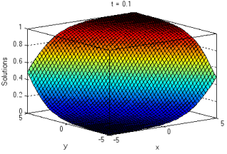
Figure 1. show the physical behavior of the solutions at different range of and for t=0.1.
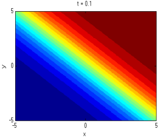
Figure 2.
Shows the contour diagram of the solutions at different range of and fort=0.1.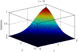
Figure 3.
Shows the physical behavior of the solutions at different range of and for t=10.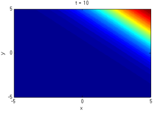
Figure 4.
Shows the contour diagram of the solutions at different range of and for t=10.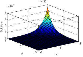
Figure 5.
Shows the physical behavior of the solutions at different range of and for t=30.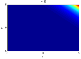
Figure 6.
Shows the contour diagram of the solutions at different range of and for t=30.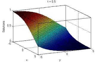
Figure 7.
Shows the physical behavior of the solutions at different range of ,and z = 0.5 for t=0.5.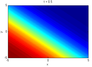
Figure 8. Shows the contour diagram of the solutions at different range of , and z = 0.5 for t=0.5.
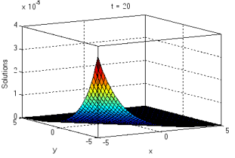
Figure 9.
Shows the physical behavior of the solutions at different range of ,and z = 0.5 for t=20.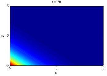
Figure 10.
Shows the contour diagram of the solutions at different range of , and z = 0.5 for t=20.Information