Time Series Analysis of Rainfall Distribution in Gambella Meteorological Station

Elias Mengst Yayeh; Abiyot Abebaw; Gashaw Setie

doi:doi:10.11648/j.ajme.20261201.11

Research Article |

| Peer-Reviewed

Time Series Analysis of Rainfall Distribution in Gambella Meteorological Station

Elias Mengst Yayeh^*

, Abiyot Abebaw

, Gashaw Setie

Published in American Journal of Modern Energy (Volume 12, Issue 1)

Received: 11 December 2025 Accepted: 6 January 2026 Published: 27 January 2026

Views: Downloads:

Download PDF

Share This Article

Twitter
Linked In
Facebook

Abstract

This study conducted on this research on the Time Series Analysis of rainfall distribution in Gambella meteorological station. On this study, we try to see what the rainfall behavior of Gambella meteorological station seems like. In our study we have used time series model and focused on time series component, to deal variation and trend of rain fall distribution in Gambella metrological station, First, we have seen the actual data of rainfall in mm of the last ten years. The data shows a little change the year. When we see the trend value of the last ten years of the rain it is proportionally a little increasing. From the seasonal indices we have seen there was higher rainfall in the beginning of the years that means the earliest time and it shows proportionally decreasing except 2009 was higher rainfall. Lastly we seen the forecasted value for 2013 based on the rainfall of 2012 rainfall and the forecasted value of rainfall in Gambella meteorological is similar to that of its preceding years, but it will show a little decreasing at the beginning of the year and it will be constant.

Published in	American Journal of Modern Energy (Volume 12, Issue 1)
DOI	10.11648/j.ajme.20261201.11
Page(s)	1-8
Creative Commons	This is an Open Access article, distributed under the terms of the Creative Commons Attribution 4.0 International License (http://creativecommons.org/licenses/by/4.0/), which permits unrestricted use, distribution and reproduction in any medium or format, provided the original work is properly cited.
Copyright	Copyright © The Author(s), 2026. Published by Science Publishing Group

Keywords

Rain Fall Distribution, Forecasting, Component of Time Series

1. Introduction

The western part of Ethiopia has one rainfall peak during the year

[1]

. The length of the rainy period decreases, and the length of the dry period increases as one goes toward the north within this region, as a result of that meridional migration of the occurrence of the dry spell has a particular relevance for rain-fed agriculture, as rainfall water is one of the major requirements for plant life in rain-fed agriculture. As we know, rainfall is very essential for living and non-living things. However, sometimes it may cause to a great disaster, this happens usually from the unexpected floods and unpredictable rainfall in the agriculture area and other places. Considering this, we try to predict the future trend of rainfall to analysis average variations of rainfall for ten years and to the amount of rainfall distributions in Gambella.

The inter-annual shift of the position of inter-tropical convergence zone causes variation in the wind flow patterns around and over Ethiopia. In its movement to the north and south of the equator alternatively, the ITCZ passes over Ethiopia twice a year and its seasonal migration causes rainfall to variable and seasonal in Ethiopia. The central and most of the eastern half of the country have two rainy periods and one dry period

[2]

. The two rainy periods are locally known as Kiremt (summary) (June to September) and Belg (Spring) (February to May), which are the long and short rainy periods respectively. The annual rainfall distribution over this region shows two peaks corresponding to the two rainy seasons, separated by relatively short dry period. The dry period, which covers the rest of the year (that is October to January), is known as bega

[3]

2. Methodology

2.1. Source of Data

Source of the data is secondary providing by Gambella meteorological station. This study was based on the amount of monthly rainfall distributions in Gambella meteorological station for ten years.

2.2. Variable Under Study

Dependent variable: the amount of rainfall in mm Independent Variable: (Time month, seasons, years) In this study, the dependent variable is the amount of rainfall in mm and the independent variable is time (months, seasons and years). To apply Time series analysis, we have to check whether the data is time dependent (random). If the data is non- random, we can apply time series analysis. There are different methods to test randomness of the data such as Rank test, Phase length test and turning point test. However, in this study we see only turning point test

[4]

Turning Point Test

The test is based on by counting the number of peaks or troughs, which it exhibits. A “peak” is a value less than its two neighboring values: a “trough”, conversely, is a value less than its two neighbors are? The two together are known as “turning points”. We consider a finite series of n values, x₁, x₂,….x_n. The initial value cannot consider (be regarded) as defining a turning point because we do not know xo, and similarly, neither can the last value since we do not know x_n+1. Three consecutive values are required to determine a turning point

[5]

. If the series is random, these three values could have arisen in any of 3! Possible orders with equal probability. In only three of these would there be a turning point, namely when the greatest or the least of three in the middle. The probability of finding a turning point in any set of three values is then 2/3.

For the set of ‘n’ values, define a counting variable y as 1, xi < xi+1 >xi+2 or x i >xi+1 <xi+2

1, xi< xi+1> xi+2 or xi> xi+1< xi+2

\{\begin{matrix} 0 \\ otherwise \end{matrix}

The number of turning point p in the series is then if n is large, the distribution of p is approximately normal with mean and variance.

The hypothesis is testing as follow

H₀: the series is random

H₁: the series is non-random

We reject H₀ at ά level of significance, if |Zcal| > Zα/2

2.3. Component of Time Series

When the data was arranged on the basis of their occurrence, we found that the variables under investigation are fluctuating from time to time. The fluctuations are cause by composite force that is constantly at work. This force has four components secular trend, cyclical variation, seasonal component and irregular or random movement

[6]

2.3.1. Seasonal Trend

Seasonal variation is short-term oscillation around the trend line. Consumption and production of many commodities, interest rates, bank clearings, etc are marked seasonal swings. Climate and custom together play an important role in giving rise to seasonal movement to all the industries.

2.3.2. Cyclical Variation

It refers to long-term oscillation about trend. In a large number of time series of economic data, it was observed that there was somewhat periodic up and down movement. Cycles in general exhibit semi-regular periodicity as these are neither as regular as are seasonal variations nor as accidental as are accidental as are the random fluctuation

[7]

2.4. Models of Time Series

There are two mathematical models, which is commonly used for the decomposition of a time series into component parts. These are additive model and multiplicative model.

Additive model

The data is the sum of the time series components. If the time series data does not contain one of the components the value for that component is equal to zero.

Symbolically

Xt = Mt + St +Ct + Et, Where Xt =observation at time t Mt = trend component at time t St= seasonal component at time t Ct= cyclical component at time t Et= random component at time t.

It is an appropriate model if we assume that all components are independent of one another and the magnitude of the seasonal fluctuations does not vary with level of the series

[8]

2.5. Estimation of Trend

The study of trend enables us to have a general idea about the pattern of the phenomena under consideration. This helps in forecasting and planning future operations

[6]

. Trend analysis enables us to compare two or more-time series over different periods of time and draw important conclusions about them. We estimate the trend by using different methods such as free hand method, selected point methods, semi-average method, moving average, method of simple exponential smoothing and the method of least squares.

2.5.1. The Least Square Point Estimates

Let b₀, b₁...., bp denote point estimates of the parameters B₀, B₁, B₂, Bp in the linear regression model Then the point prediction of (Here, I predict ei to be zero). next, for i=1, 2…n, the residual ei =Yi- yi and we are also defining the sum of squared residuals to be: Intuitively, if any particular values of b₀, b₁, b₂, ……bp are good point estimates, they will make (for i=1, 2…., n) the predicted value yi fairly close to the observed value Y and thus will make SSE fairly small

[9]

. We define the least squares point estimates to be the values of b₀, b₁, b₂, bp that minimize SSE. It can be shown that the lines regression model can be calculating by using a formula that is expressed by using mathematics called matrix algebra. Rather than present this formula, we rely on computer packages to find the least squares point estimates

[8]

2.5.2. Estimation of Seasonal Variation

For additive model (simple moving average) Among all methods of measuring seasonal variation, this method is the most satisfactory and widely used. In this method, we first subtract the trend value obtain by least squares method from the actual data (i. eYt-Mt = Ct + St + Et). When these deviations from trend will average for each month, the cyclic and irregular components is remove to a large extent. The only component left is seasonal which is suitable to adjust so as to be total zero

[10]

The adjustment is in the following way: Adjustment=General average with sign reversed.

Seasonal index= Average for each month + Adjustment

2.5.3. Measurement of Cyclical Variation

We can estimate cyclical variation using various methods. But, we consider only residual method. For additive model First depersonalize the data, Xt_St=Mt +Ct +Et.Then from the quantity that will obtain subtract trend estimate, Xt_St_Mt=Ct +Et. Finally, take an appropriate moving average of the periods to take the effect of irregular component. The remaining data is the estimate of cyclical component

[11]

2.6. Forecasting a Time Series Data

Forecasting will be prediction of future values of certain variable. The study of the behavior of variable enables to predict future tendencies

[12]

. To business executives who are to plan their production program such analysis is, therefore, of great assistance, for it with the help of analysis of this nature that appropriately correct estimates of the future demand will be make. There will be several forecasting methods such as average method, classical model decomposition, exponential smoothing, least squares method, econometric and Box-Jenkins methods. However, in this study we consider classical model decomposition

[13]

3. Results

In this chapter we analyze the data of monthly rainfall amount in mm of Gambella meteorological station starting from January 1993 to December 2012.

The data is shown in Table 1 and in Figure 1.

Test of randomness.

Ho: the series is random. H1: the series is not random.

Level of significance α=0.05 Test statistics Z =

\frac{P - E (P)}{\sqrt{VAR (P)}}

Where P is the number of turning points P = 75

n = 120, n = number of observation

E (P) = \frac{2}{3} (n - 3) = \frac{2}{3} (120 - 3)

E (P) = 7 Var (P) = \frac{16120 - 29}{90} = \frac{16 x 120 - 29}{90} = 21.011

Z = \frac{75 - 78}{\sqrt{21.011}} = 1.965

The critical value is Z_α/2 = 1.96 Decision: /Z_cal / > Z_α/2 that is /1.965/ > 1.96 then reject H_O. Therefore, we conclude that the data seems to time dependent.

3.1. Model of Time Series

When we plot the time series data shown in Figure 1, the variability of the data is constant through time. Therefore, the appropriate additive model for our data. i.e. Xt = Mt + St + Ct + Et, Where Mt = trend component at time t St=seasonal component at time t Ct=cyclical component at time t Et=random component at time.

Table 1. The actual data on monthly rainfall for Gambella meteorological station in mm. The actual data on monthly rainfall for Gambella meteorological station in mm. The actual data on monthly rainfall for Gambella meteorological station in mm.

Year	Jan	Feb	Mar	Apr	May	Jun	Jul	Aug	Sep	Oct	Nov	Dec
2003	28.8	61.5	87.4	116	22.3	266.2	186.9	145	239	91.8	30	14.6
2004	51.2	12.4	46.2	130.6	162.2	165.7	216.6	219.2	201	133.3	67.5	81.1
2005	44.5	0.5	193.8	141.7	173	176.8	273.6	237.6	229	68.3	29.7	0.0
2006	16.2	77.2	181.8	110.7	211.7	207.6	327.6	240.3	169.9	91.4	127.9	100.5
2007	37.7	51.4	104.3	121.7	226.1	138.4	247.5	177.4	256.3	51	5.9	0.0
2008	34.1	12.3	39.4	108.7	247.2	238.4	221.2	236.9	133.5	191.2	.4	6.3
2009	63.2	29.5	80.1	103.7	244.6	160.3	149.8	304.7	199.5	92.4	78.5	58.2
2010	27.3	88.4	-67.7	101.4	193	394.7	181.3	203.4	186.7	57.9	94.9	7.7
2011	24.4	6.2	34.4	151.1	182.9	311.2	199.9	.190.8	269.7	11	105	25.1
2012	2.2	1.9	55.9	154.5	119	335	223.9	132.8	250.6	32.8	77.4	58

Download: Download full-size image

Figure 1. Shows the actual data on monthly rainfall for Gambella meteorological station. Shows the actual data on monthly rainfall for Gambella meteorological station.

As we see from the graph the amount of rainfall change based on the time because there is variation from time to time. The graph shows as the rainfall is high at the middle of the years and there are very high in summer season.

3.2. Estimation of Trend

We compute the estimated trend value by using least square method. To know the appropriate regression model; we have to compare MAD for linear and quadratic model. The data at hand seems to follow quadratic model because for linear model MAD=50.99, but for quadratic model, MAD=50.81.

Applying the least square method, we fitted linear equation, which is given by Yt=bo+b1t+Et.where, bo and b1t are intercept and slope of the model respectively; Et represents the random deviation from the mean. The estimated semiannual trend value is given by the equation Yt=62.7059+0.55t-4.36t² where, t=1, 2…, 40 Time unit: one-month Origin: Jan 2003 By using the equation and substitute the appropriate time t, we found the estimated trend value for each month of rain fall. It is shown in Table 2 and Figure 2.

Download: Download full-size image

Figure 2. The estimated trend value by using least square method. The estimated trend value by using least square method.

From the graph we can see that the trend line shows there is increasing pattern in rain fall with respect to time, but at the end it shows a little decreasing. From the graph we can see that the trend line shows there is increasing pattern in rain fall with respect to time, but at the end it shows a little decreasing. At the middle there are high amount of the rainfall then at the beginning and end. From this we concluded the amount of rain is a little at bega (autumn).

Table 2. The estimated trend value of rainfall in Gambella meteorological station in mm.The estimated trend value of rainfall in Gambella meteorological station in mm.The estimated trend value of rainfall in Gambella meteorological station in mm.

Year	Jan	Feb	Mar	Apr	May	Jun	Jul	Aug	Sep	Oct	Nov	Dec
2003	63.25	63.79	64.32	64.84	65.35	65.85	66.34	66.83	67.31	67.77	68.23	68.68
2004	69.12	69.56	69.98	70.39	70.80	71.20	71.59	71.97	72.34	72.70	73.06	73.40
2005	73.74	74.07	74.38	74.69	75.00	75.29	75.57	75.85	76.12	76.37	76.62	76.86
2006	77.09	77.32	77.53	77.74	77.93	78.12	78.30	78.47	78.64	78.79	78.93	79.07
2007	79.20	79.31	79.42	79.52	79.62	79.70	79.77	79.84	79.90	79.95	79.99	80.02
2008	80.04	80.05	80.06	80.05	80.04	80.02	79.99	79.95	79.90	79.85	79.78	79.71
2009	79.63	79.54	79.44	79.33	79.21	79.08	78.95	78.81	78.65	78.49	78.32	78.14
2010	77.96	77.76	77.56	77.34	77.12	76.89	76.65	76.40	76.15	75.88	75.61	75.32
2011	75.03	74.73	74.42	74.10	73.78	73.44	73.10	72.74	72.38	72.01	71.63	71.24
2012	70.85	70.44	70.03	69.61	69.17	68.73	68.29	67.83	67.36	66.89	66.40.	65.91

This table indicates the estimated value of trend values of rainfall for ten years by using least square method and from the table the distribution of rainfall not so much different in a short period, but it shows a little change through time.

3.2.1. Estimation of Seasonal Variation

Applying the method of ratio moving average method to the serious, we obtain seasonal indices for monthly rainfall amount in mm of Gambella meteorological station.

Table 3. The estimated seasonal indices of rainfall in mm.The estimated seasonal indices of rainfall in mm.The estimated seasonal indices of rainfall in mm.

Year	Jan	Feb	Mar	Apr	May	Jun	Jul	Aug	Sep	Oct	Nov	Dec
2003	-	-	-4.39	.34	-1.38	-18.63	-27.20	--18.76	-18.97	-4.30	5.79	-13.06
2004	-17.17	-7.50	18.80	51.79	58.78	42.88	12.10	-7.86	-9.56	-21.52	-32.66	-39.67
2005	-47.98	-30.19	-9.24	-6.66	-5.62	-16.98	-25.89	-20.42	-2.72	7.65	-3.66	-17.01
2006	-33.27	-7.87	51.07	76.98	74.04	33.16	-20.94	-25.89	-12.26	-13.93	-24.25	-36.91
2007	-28.49	-1.60	26.90	46.80	37.97	18.82	2.94	-3.86	10.07	25.36	33.36	20.54
2008	-5.63	-15.05	2.55	27.76	48.57	56.65	57.01	57.28	47.13	28.43	-12.20	-48.84
2009	-57.42	-40.73	-17.89	-3.54	1.91	-10.89	-.80	28.28	39.29	34.18	6.82	-31.89
2010	-52.23	-41.92	-21.5 6	-11.94	-14.6	-29.20	-47.94	-37.99	-17.99	-5.43	2.76	-14.00
2011	-5.91	24.90	60.41	90.99	75.93	39.55	10.61	.15	-3.30	-10.87	-31.84	-57.1
2012	-62.76	-58.78	-23.46	13.66	18.01	25.73	4.80	-16.30	-7.81	-3.49	-	-

Seasonal index (1473.84, 8151.477, -350.127, 12075.105, -12387.342, -5969.62, 1489.873, 6448.523, -1007.6, -2721.941, 2618.143, 1159.49)

The table indicates the estimated values seasonal variations of rainfall. The table indicate to us the rainfall is increasing or decreasing with respect to time or its various from seasons to seasons especially in summer and spring (belg). There was proportionally high rainfall at the first three years and the last four years, but at the middle of the years there was relatively low rainfall.

Download: Download full-size image

Figure 3. Graph of the seasonal indices of rainfall in Gambella meteorological station. Graph of the seasonal indices of rainfall in Gambella meteorological station.

From the graph and the table, we can see that there was proportionally high rain fall at the first three years and the last four years, but at the middle years there was relatively low rainfall. The figure indicates to us the rainfall is increasing or decreasing with respect to time or its various from seasons to seasons especially in summer and spring (belg) there is high amount of rainfall this is why our graphs are increasing up at the first three years and at the last of the years.

3.2.2. Estimation of Cyclical Variation

We can estimate cyclical variation using various methods. But, we consider only residual method.

Table 4. The estimated value of cyclical variation.The estimated value of cyclical variation.The estimated value of cyclical variation.

Year	Jan	Feb	Mar	Apr	May	Jun	Jul	Aug	Sep	Oct	Nov	Dec
2003					-13.07	-27.00	-48.64	-54.59	-39.44	-32.01	-31.73	-26.60
2004	-4.07	18.35	37.41	41.74	29.26	24.18	22.12	15.81	2.15	-8.03	-9.72	-11.22
2005	-9.05	-5.00	-1.80	3.63	9.48	8.10	4.33	-.27	-3.37	-5.39	-17.43	-20.05
2006	- 16.92	-15.3	-10.51	-5.61	-.75	2.69	12.38	6.44	-8.15	-9.50	-8.72	-7.71
2007	-3.32	7.92	15.01	22.18	31.81	33.94	33.76	38.09	40.99	33.36	27.10	24.63
2008	24.30	26.35	30.72	31.96	28.18	20.42	5.07	-4.90	-10.65	-16.20	-23.12	-31.16
2009	- 35.72	-31.5	-15.47	-6.07	.15	10.27	13.79	12.46	11.13	9.61	8.26	6.45
2010	.22	-8.06	-12.75	-12.70	-12.02	-7.64	-12.13	-17.28	-15.49	-16.98	-15.71	-14.53
2011	- 13.35	-11.10	-.20	9.65	15.38	18.40	13.48	6.85	-.48	-10.89	-25.69	-39.09
2012	-36.62	-23.06	-16.42	-7.27	3.24	6.84	10.53	22.81

The tables indicate to us the estimated value of rain is increasing or decreasing with the respect to time. The amount of rainfall is high in the middle of 2007 and 2008 and also high at the middle of the last year.

Download: Download full-size image

Figure 4. Cyclical variation. Cyclical variation.

The graph indicates to us the estimated value of rain is increasing or decreasing with the respect to time i.e its graph is cyclically up and down at the beginning, at middle and also near the last it cyclically up and down. The amount of rainfall is high near the beginning, at middle and high at the middle of the last years.

3.3. Forecasting

According to the study we got monthly forecasted rainfall amount of Gambella meteorological station for 2013

[14]

. First checking stationary of the data by using difference method and then we have got stationary time series data we see from the given graph. The graph shows there is no variability between the observation. From the box-Jenkins model we take the mixed model that is ARIMA (autoregressive integrated moving average) method with order of (p,d,q).As we said the observation have no difference (d=0) then the remaining of the model is ARMA(p,q).

3.3.1. Stationarity Checking Graph

Yt=Ф1Yt-1+Ф2Yt-2++ФpYt-p+εt-ө1εt-1-ө2εt-2-….-өqεt-q

That is autoregressive is order two and moving average is order four the difference is zero.

Then our model is given by: Yt= Ф 1Yt-1+ Ф 2 Yt-2+ Ф t-ө1 ε t-1- ө2 ε t-2- ө3 ε t-3- ө3 ε t-4

We have the estimated value of the parameters, Final Estimates of Parameters.

Download: Download full-size image

Figure 5. Stationarity checking graph. ARMA(p,q). Stationarity checking graph. ARMA(p,q).

Table 5. Estimates of Parameters. Estimates of Parameters. Estimates of Parameters.

Type		Coef	SE Coef	T	P
AR	1	-0.2129	0.2891	-0.74	0.463
AR	2	0.2550	0.2722	0.94	0.351
MA	1	-0.4690	0.2764	-1.70	0.092
MA	2	0.2709	0.2436	1.11	0.269
MA	3	0.3527	0.1142	3.09	0.003
MA	4	0.3206	0.0992	3.23	0.002

3.3.2. Test of Significance for the ARIMA Parameter

The values of the parameter Ф 1, Ф 2, ө1, ө2 are not significance, since α value is less than p-value then we ignored them as a result the model is formed by the remaining parameter

[15]

Yt=εt-0.3527εt-3-0.3206εt-4

The value of parameter ө3, and ө4 are significance, since p value is less than α value.

From the given model we forecast the 2013 rainfall of Gambella meteorological station in mm based on 2012 rainfall.

Table 6. Forecasted value of rainfall in Gambella meteorological station in mm. Forecasted value of rainfall in Gambella meteorological station in mm. Forecasted value of rainfall in Gambella meteorological station in mm.

2013	Jan	Feb	Mar	Apr	May	Jun	Jul	Aug	Sep	Oct	Nov	Dec
forecasted value	92.70	81.10	78.43	64.14	78.47	71.77	76.85	74.10	75.95	74.84	75.56	75.12

Download: Download full-size image

Figure 6. Forecasted value of rainfall in Gambella meteorological station in mm. Forecasted value of rainfall in Gambella meteorological station in mm.

From the forecasted data we concluded that there will be a little decreasing at the beginning of the years and then it will be uniform beginning from May, the relation between the forecasted rainfall and the previous rainfall is almost similar behavior that is there is no difference. From the graph of forecasting, the future amount of the rainfall is not so much different from the previous amount of the rainfall. This indicate that there is a little change for rainfall in Gambella.

4. Conclusion

In this study, we have discussed time series analysis on monthly amount of rainfall in Gambella meteorological station. Before applying time series analysis firstly, we have tested whether the data is time dependent (not random) or time independent (random) by using turning point test. Moreover, the data seem to be time dependent.

After we measured different components of time series, first we tried to identify the characteristics of trend using the method of least square. Then we measured the seasonal variation by the method of simple moving average. As we see from Figure 3, there was lower rainfall in the middle of the given years and there was relatively higher rainfall. We also measured the cyclical variation of the data by using residual method. Finally, we tried to forecast the next year monthly rainfall amount in mm of Gambella meteorological station.

5. Recommendation

1) The rain fed agriculture in Gambella should be supplemented by rainfall. These are not sufficient for their development. Therefore, they should have to use irrigation in addition to the rainfall to achieve successive development in a few.

2) Since deforestation cause, the decreasing of rainfall every person of the zone should has to plant the trees in order to keep the air condition of their environment from the desert.

3) It is better for farmers to construct the terracing to conserve the soil from erosion as well as ploughing horizontally, when high amount of rainfall is raining. By doing this they can support the economy of the region and they can resist drought.

Abbreviations

AR	Autoregressive
MA	Moving Average
ARIMA	Autoregressive Integrated Moving Average

Conflicts of Interest

The authors declare no conflicts of interest.

References

[1]	N. R. The Nile River Basin ecohydrology system: Problems and solutions.
[2]	C. Palomares-salas, J. Jose, G. Ramiro-leo, A. Moreno-mun, "Journal of Wind Engineering Basic meteorological stations as wind data source : A mesoscalar test $", ELSEVIER, 108, 48-56, 2012.
[3]	S. Wales, B. Harman, R. Cunningham, B. Jacobs, T. Measham, C. Cvitanovic, "Engaging local communities in climate adaptation : a social network perspective from Bega Valley, New", May 2015.
[4]	L. J. Christiano, "Christopher A. Sims and Vector",. 114, 4, 2012,. 1082-1104. https://doi.org/10.1111/j.1467-9442.2012.01737.x
[5]	J. H. Stock M. W. Watson, "ESTIMATING TURNING POINTS USING LARGE DATA SETS", Harvard Univ., 2010.
[6]	A. Harvey, "FORECASTING WITH UNOBSERVED COMPONENTS TIME SERIES MODELS", 1, 05, 2006, https://doi.org/10.1016/S1574-0706(05)01007-4
[7]	Y. S. Schüler و P. P. Hiebert, "Working Paper Series a multivariate and time-varying", Eur. CENTERAL BANK, 2015.
[8]	G. L. Simpson, "Modelling Palaeoecological Time Series Using Generalised Additive Models", Frontiers (Boulder)., 6, October, 1-21, 2018, https://doi.org/10.3389/fevo.2018.00149
[9]	P. Simmonds, "SSE : a nucleotide and amino acid sequence analysis platform SSE : a nucleotide and amino acid sequence analysis platform", Springer,. 50, January, 2012.
[10]	B. Berhanu, Y. Seleshi, A. M. Melesse, "Surface Water and Groundwater Resources of Ethiopia : Potentials and Challenges of Water Resources Development", https://doi.org/10.1007/978-3-319-02720-3
[11]	N. B. Ellison, "Social network sites and society: Current trends and future possibilities", Interactions, 16, 1, 6-9, 2009, https://doi.org/10.1145/1456202.1456204
[12]	S. Gonzales Chavez, J. Xiberta Bernat, H. Llaneza Coalla, "Forecasting of energy production and consumption in Asturias (northern Spain)", Energy, 24,. 183-198, 1999, https://doi.org/10.1016/S0360-5442(98)00099-1
[13]	Z. Girma, "Success, Gaps and Challenges of Power Sector Reform in", Am. J. Mod. Energy, 6, 1, 33-42, 2020, https://doi.org/10.11648/j.ajme.20200601.15
[14]	G. P. Zhang و M. Qi, "Neural network forecasting for seasonal and trend time series", 160, 501-514, 2005, https://doi.org/10.1016/j.ejor.2003.08.037
[15]	R. I. D. Harris, "Testing for unit roots using the augmented Dickey-Fuller test. Some issues relating to the size, power and the lag structure of the test", Econ. Lett., 38, 381-386, 1992, https://doi.org/10.1016/0165-1765(92)90022-Q

Cite This Article

Plain Text BibTeX RIS

APA Style

Yayeh, E. M., Abebaw, A., Setie, G. (2026). Time Series Analysis of Rainfall Distribution in Gambella Meteorological Station. American Journal of Modern Energy, 12(1), 1-8. https://doi.org/10.11648/j.ajme.20261201.11

Copy | Download

ACS Style

Yayeh, E. M.; Abebaw, A.; Setie, G. Time Series Analysis of Rainfall Distribution in Gambella Meteorological Station. Am. J. Mod. Energy 2026, 12(1), 1-8. doi: 10.11648/j.ajme.20261201.11

Copy | Download

AMA Style

Yayeh EM, Abebaw A, Setie G. Time Series Analysis of Rainfall Distribution in Gambella Meteorological Station. Am J Mod Energy. 2026;12(1):1-8. doi: 10.11648/j.ajme.20261201.11

Copy | Download

@article{10.11648/j.ajme.20261201.11,
  author = {Elias Mengst Yayeh and Abiyot Abebaw and Gashaw Setie},
  title = {Time Series Analysis of Rainfall Distribution in Gambella Meteorological Station},
  journal = {American Journal of Modern Energy},
  volume = {12},
  number = {1},
  pages = {1-8},
  doi = {10.11648/j.ajme.20261201.11},
  url = {https://doi.org/10.11648/j.ajme.20261201.11},
  eprint = {https://article.sciencepublishinggroup.com/pdf/10.11648.j.ajme.20261201.11},
  abstract = {This study conducted on this research on the Time Series Analysis of rainfall distribution in Gambella meteorological station. On this study, we try to see what the rainfall behavior of Gambella meteorological station seems like. In our study we have used time series model and focused on time series component, to deal variation and trend of rain fall distribution in Gambella metrological station, First, we have seen the actual data of rainfall in mm of the last ten years. The data shows a little change the year. When we see the trend value of the last ten years of the rain it is proportionally a little increasing. From the seasonal indices we have seen there was higher rainfall in the beginning of the years that means the earliest time and it shows proportionally decreasing except 2009 was higher rainfall. Lastly we seen the forecasted value for 2013 based on the rainfall of 2012 rainfall and the forecasted value of rainfall in Gambella meteorological is similar to that of its preceding years, but it will show a little decreasing at the beginning of the year and it will be constant.},
 year = {2026}
}

Copy | Download

TY  - JOUR
T1  - Time Series Analysis of Rainfall Distribution in Gambella Meteorological Station
AU  - Elias Mengst Yayeh
AU  - Abiyot Abebaw
AU  - Gashaw Setie
Y1  - 2026/01/27
PY  - 2026
N1  - https://doi.org/10.11648/j.ajme.20261201.11
DO  - 10.11648/j.ajme.20261201.11
T2  - American Journal of Modern Energy
JF  - American Journal of Modern Energy
JO  - American Journal of Modern Energy
SP  - 1
EP  - 8
PB  - Science Publishing Group
SN  - 2575-3797
UR  - https://doi.org/10.11648/j.ajme.20261201.11
AB  - This study conducted on this research on the Time Series Analysis of rainfall distribution in Gambella meteorological station. On this study, we try to see what the rainfall behavior of Gambella meteorological station seems like. In our study we have used time series model and focused on time series component, to deal variation and trend of rain fall distribution in Gambella metrological station, First, we have seen the actual data of rainfall in mm of the last ten years. The data shows a little change the year. When we see the trend value of the last ten years of the rain it is proportionally a little increasing. From the seasonal indices we have seen there was higher rainfall in the beginning of the years that means the earliest time and it shows proportionally decreasing except 2009 was higher rainfall. Lastly we seen the forecasted value for 2013 based on the rainfall of 2012 rainfall and the forecasted value of rainfall in Gambella meteorological is similar to that of its preceding years, but it will show a little decreasing at the beginning of the year and it will be constant.
VL  - 12
IS  - 1
ER  -

Copy | Download

Author Information

Elias Mengst Yayeh

Department of Statistics, Gambella University, Gambella, Ethiopia

Contact Email

http://orcid.org/0009-0007-0905-4215
Abiyot Abebaw

Department of Statistics, Gambella University, Gambella, Ethiopia

Contact Email

http://orcid.org/0009-0009-6253-9806
Gashaw Setie

Department of Statistics, Gambella University, Gambella, Ethiopia

Contact Email

http://orcid.org/0009-0007-8649-2243

Download PDF

Submit an Article

Figure 1

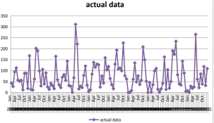
Figure 1. Shows the actual data on monthly rainfall for Gambella meteorological station.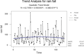
Figure 2

Figure 2. The estimated trend value by using least square method.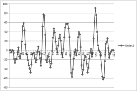
Figure 3

Figure 3. Graph of the seasonal indices of rainfall in Gambella meteorological station.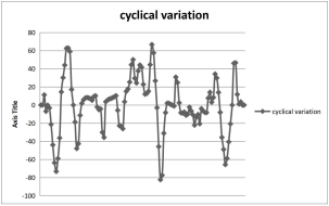
Figure 4

Figure 4. Cyclical variation.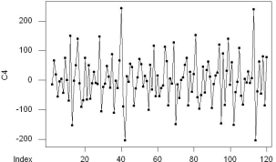
Figure 5

Figure 5. Stationarity checking graph. ARMA(p,q).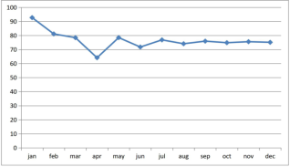
Figure 6

Figure 6. Forecasted value of rainfall in Gambella meteorological station in mm.

Table 1

Table 1. The actual data on monthly rainfall for Gambella meteorological station in mm. The actual data on monthly rainfall for Gambella meteorological station in mm.
Table 2

Table 2. The estimated trend value of rainfall in Gambella meteorological station in mm.The estimated trend value of rainfall in Gambella meteorological station in mm.
Table 3

Table 3. The estimated seasonal indices of rainfall in mm.The estimated seasonal indices of rainfall in mm.
Table 4

Table 4. The estimated value of cyclical variation.The estimated value of cyclical variation.
Table 5

Table 5. Estimates of Parameters. Estimates of Parameters.
Table 6

Table 6. Forecasted value of rainfall in Gambella meteorological station in mm. Forecasted value of rainfall in Gambella meteorological station in mm.

Plain Text BibTeX RIS

APA Style

Yayeh, E. M., Abebaw, A., Setie, G. (2026). Time Series Analysis of Rainfall Distribution in Gambella Meteorological Station. American Journal of Modern Energy, 12(1), 1-8. https://doi.org/10.11648/j.ajme.20261201.11

Copy | Download

ACS Style

Yayeh, E. M.; Abebaw, A.; Setie, G. Time Series Analysis of Rainfall Distribution in Gambella Meteorological Station. Am. J. Mod. Energy 2026, 12(1), 1-8. doi: 10.11648/j.ajme.20261201.11

Copy | Download

AMA Style

Yayeh EM, Abebaw A, Setie G. Time Series Analysis of Rainfall Distribution in Gambella Meteorological Station. Am J Mod Energy. 2026;12(1):1-8. doi: 10.11648/j.ajme.20261201.11

Copy | Download

@article{10.11648/j.ajme.20261201.11,
  author = {Elias Mengst Yayeh and Abiyot Abebaw and Gashaw Setie},
  title = {Time Series Analysis of Rainfall Distribution in Gambella Meteorological Station},
  journal = {American Journal of Modern Energy},
  volume = {12},
  number = {1},
  pages = {1-8},
  doi = {10.11648/j.ajme.20261201.11},
  url = {https://doi.org/10.11648/j.ajme.20261201.11},
  eprint = {https://article.sciencepublishinggroup.com/pdf/10.11648.j.ajme.20261201.11},
  abstract = {This study conducted on this research on the Time Series Analysis of rainfall distribution in Gambella meteorological station. On this study, we try to see what the rainfall behavior of Gambella meteorological station seems like. In our study we have used time series model and focused on time series component, to deal variation and trend of rain fall distribution in Gambella metrological station, First, we have seen the actual data of rainfall in mm of the last ten years. The data shows a little change the year. When we see the trend value of the last ten years of the rain it is proportionally a little increasing. From the seasonal indices we have seen there was higher rainfall in the beginning of the years that means the earliest time and it shows proportionally decreasing except 2009 was higher rainfall. Lastly we seen the forecasted value for 2013 based on the rainfall of 2012 rainfall and the forecasted value of rainfall in Gambella meteorological is similar to that of its preceding years, but it will show a little decreasing at the beginning of the year and it will be constant.},
 year = {2026}
}

Copy | Download

TY  - JOUR
T1  - Time Series Analysis of Rainfall Distribution in Gambella Meteorological Station
AU  - Elias Mengst Yayeh
AU  - Abiyot Abebaw
AU  - Gashaw Setie
Y1  - 2026/01/27
PY  - 2026
N1  - https://doi.org/10.11648/j.ajme.20261201.11
DO  - 10.11648/j.ajme.20261201.11
T2  - American Journal of Modern Energy
JF  - American Journal of Modern Energy
JO  - American Journal of Modern Energy
SP  - 1
EP  - 8
PB  - Science Publishing Group
SN  - 2575-3797
UR  - https://doi.org/10.11648/j.ajme.20261201.11
AB  - This study conducted on this research on the Time Series Analysis of rainfall distribution in Gambella meteorological station. On this study, we try to see what the rainfall behavior of Gambella meteorological station seems like. In our study we have used time series model and focused on time series component, to deal variation and trend of rain fall distribution in Gambella metrological station, First, we have seen the actual data of rainfall in mm of the last ten years. The data shows a little change the year. When we see the trend value of the last ten years of the rain it is proportionally a little increasing. From the seasonal indices we have seen there was higher rainfall in the beginning of the years that means the earliest time and it shows proportionally decreasing except 2009 was higher rainfall. Lastly we seen the forecasted value for 2013 based on the rainfall of 2012 rainfall and the forecasted value of rainfall in Gambella meteorological is similar to that of its preceding years, but it will show a little decreasing at the beginning of the year and it will be constant.
VL  - 12
IS  - 1
ER  -

Copy | Download