Mathematical Modeling of Tumor-Immune Interaction with Optimal Control in the Human System

Tewele Assefa Welu; Subrata Kumar Sahu; Ataklti Araya; Habtu Alemayehu; Yohannes Yirga

doi:doi:10.11648/j.sdmath.20260101.14

Research Article |

| Peer-Reviewed

Mathematical Modeling of Tumor-Immune Interaction with Optimal Control in the Human System

Tewele Assefa Welu^*, Subrata Kumar Sahu, Ataklti Araya, Habtu Alemayehu, Yohannes Yirga

Published in Science Discovery Mathematics (Volume 1, Issue 1)

Received: 6 February 2026 Accepted: 2 March 2026 Published: 12 March 2026

Views: Downloads:

Download PDF

Share This Article

Twitter
Linked In
Facebook

Abstract

This paper presents a mathematical analysis of the immune response to tumor growth, conceptualized through the lens of predator-prey interactions. We investigate a three-dimensional mathematical model that captures the complex dynamics between tumor cells (the prey), hunting immune cells (active predators), and resting immune cells (reservoir population). The model extends classical ecological frameworks to immunology, recognizing that tumors and immune cells engage in a continuous battle for survival within the human body much like species competing in an ecosystem. We first establish the biological validity of our model by proving that all solutions remain positive, exist uniquely, and stay bounded over time essential properties when modeling living systems where negative populations would make no sense. Our analysis reveals that this seemingly simple system harbors surprisingly rich dynamical behavior. Unlike earlier models based on mass-action kinetics, our formulation shows the existence of multiple equilibrium points, representing different disease outcomes: tumor elimination, uncontrolled growth, or chronic persistence. Most notably, we identify conditions under which Hopf bifurcations occur, giving rise to limit cycles periodic oscillations in tumor and immune cell populations that mirror clinical observations of cancer remission and relapse cycles. Recognizing that clinical reality demands more than just understanding these dynamics, we implement a feedback control strategy designed to stabilize tumor populations at clinically manageable levels. Rather than aiming for complete eradication (which may not always be achievable), this approach seeks to transform aggressive growth into a controlled, chronic condition. Numerical simulations demonstrate that our control mechanism can successfully stabilize otherwise unstable equilibria, effectively "taming" the tumor's behavior. Parameter sensitivity analysis reveals that the half-saturation constants play particularly crucial roles in determining system outcomes. These constants, which govern how quickly immune responses saturate with increasing tumor burden, emerge as potential therapeutic targets. The findings suggest that treatments modifying these immunological thresholds might be as important as those directly killing tumor cells a perspective that could inform future immunotherapy strategies. This work bridges ecological modeling, dynamical systems theory, and clinical oncology, offering both theoretical insights into tumor-immune interactions and practical tools for treatment optimization.

Published in	Science Discovery Mathematics (Volume 1, Issue 1)
DOI	10.11648/j.sdmath.20260101.14
Page(s)	34-42
Creative Commons	This is an Open Access article, distributed under the terms of the Creative Commons Attribution 4.0 International License (http://creativecommons.org/licenses/by/4.0/), which permits unrestricted use, distribution and reproduction in any medium or format, provided the original work is properly cited.
Copyright	Copyright © The Author(s), 2026. Published by Science Publishing Group

Keywords

Tumor Growth, Predator-Prey, Immune System, Stability, Optimal Control, Holling Type-II Functional Response, Hopf Bifurcation

1. Introduction

Cancer is widely recognized as one of the world’s leading causes of death, making the control of tumor growth a critical global health challenge. The World Health Organization (WHO) estimates that approximately six million people die yearly due to cancer, making it the second most fatal disease after cardiovascular diseases

[30]

. Consequently, understanding tumor dynamics and developing effective therapeutic strategies is of major public health interest. Cancer begins when the tightly regulated process of cell growth and division breaks down, leading to uncontrolled cell proliferation and the formation of a mass of extra tissue called a tumor

[2, 4]

. Tumors are classified as either benign (noncancerous) or malignant (cancerous). Malignant tumors are particularly dangerous because they can invade and destroy surrounding healthy tissue and metastasize, spreading through the bloodstream or lymphatic system to form secondary tumors in distant organs

[19]

In human physiology, the immune system plays a crucial role in identifying and eliminating tumor cells when they are detectable as non-self

[32-34]

. The cellular immune response is primarily carried out by T lymphocytes, which include both resting T cells and hunting (cytotoxic) T cells

[13-17]

. Resting T cells recognize tumor antigens through major histocompatibility complex (MHC) molecules and produce cytokines, but they cannot directly kill tumor cells. These cytokines activate resting T cells to become cytotoxic T lymphocytes (hunting cells), which can eliminate tumor cells through cytotoxic reactions

[29]

The tumor microenvironment encompasses immune cells, fibroblasts, endothelial cells, the extracellular matrix, and signaling molecules including chemokines, cytokines, and growth factors

[9]

. Findings from the last two decades have evolved the conceptual framework from “immunosurveillance” referring to the immune system’s tumor-protective role to “cancer immunoediting,” which describes its dual function in both protecting against and sculpting tumors

[36, 38, 39]

Mathematical modeling has become an essential tool for understanding tumor-immune dynamics and designing therapeutic strategies

[3, 20]

. This paper investigates an ordinary differential equation model comprising three equations that describe the interactions among cancer cells and two classes of immune cells: resting and hunting T lymphocytes. The model’s structure builds upon foundational frameworks

[17, 19]

and modifies previous approaches

[10]

by substituting mass-action functional responses with Holling’s Type II response. This adjustment incorporates more biologically realistic growth dynamics and reveals novel dynamical scenarios unattainable under mass-action kinetics.

2. Model Formulation

Following the modeling methodology of previous studies

[17, 19]

, we consider a prey-predator type model for the interaction between cancer cell population (prey) and hunting and resting effector cells (predators)

[8, 10]

\frac{dT}{dt} = q + rT (1 - \frac{T}{k_{1}}) - f (T) H

\frac{dH}{dt} = g (R) H - d_{1} H

(1)

\frac{dR}{dt} = sR (1 - \frac{T}{k_{2}}) - g (R) H - d_{1} R

All model parameters are positive constants. Since cell concentrations cannot be negative, the state space of system (1) is restricted to T (t) ≥ 0, H(t) ≥ 0, and R(t) ≥ 0.

In equations (1):

1) T (t) represents the tumor cell population at time t

2) H(t) represents the hunting effector cell population at time t

3) R(t) represents the resting effector cell population at time t

4) q is the conversion rate of normal cells to malignant ones

5) r is the intrinsic growth rate of tumor cells

6) k₁ is the carrying capacity of the tumor cell population

7) α is the killing rate of tumor cells by hunting cells

8) β is the conversion rate of resting cells to hunting cells

9) d₁ is the natural death rate of hunting cells

10) s is the growth rate of resting cells

11) k₂ is the carrying capacity of resting cells

12) d₂ is the natural death rate of resting cells

13) f (T) denotes the functional response of hunting effector cells to tumor cell population

14) g(R) represents the functional response of hunting effector cells to conversion of resting effector cells

Previous studies

[10-12]

considered linear functional responses:

f (T) = αT,g(R) = βR(2)

However, these forms are not biologically realistic as they describe unlimited killing capacity of hunting effector cells and unlimited conversion capacity of resting effector cells. More realistic functional responses exhibit saturation effects

[1]

. Therefore, we modify model (1) by incorporating Holling’s Type-II functional responses:

f (t) = \frac{αT}{a + T}

and

g (t) = \frac{βR}{b + R}

(3)

Here, a represents the half-saturation population of tumor cells, the population at which the hunting effector cell’s killing capacity reaches half its maximum. Similarly, b is the half- saturation population of resting effector cells. Substituting (3) into model (1), our main model becomes:

\frac{dT}{dt} = q + rT (1 - \frac{T}{k_{1}}) - \frac{αT}{a + T} H

\frac{dH}{dt} = \frac{β}{b + R} H - d_{1} H

(4)

\frac{dR}{dt} = sR (1 - \frac{T}{k_{2}}) - \frac{β}{b + R} H - d_{2} R

Non-Dimensionalization

To reduce the number of system parameters, we introduce the following dimensionless variables:

t^{*} = \frac{qt}{k_{1}}, x_{1} = \frac{T}{k_{1}}, x_{2} = \frac{αH}{q}, x_{3} = \frac{R}{k_{2}}, c_{1} = \frac{r k_{1}}{q}, c_{2} = \frac{β}{q} k_{1}, c_{3} = \frac{k_{1}}{q} d_{1}

c_{4} = s \frac{k_{1}}{q}

c_{5} = β \frac{k_{1}}{α k_{2}}

c_{6} = \frac{{d_{2} k}_{1}}{q}, w_{1}

\frac{a}{k_{1}}

and

w_{2}

\frac{b}{k_{2}}

(5)

The biological interpretations of the dimensionless parameters are:

1) c₁: dimensionless tumor growth rate

2) c₂, c₅: dimensionless conversion rates

3) c₃, c₆: dimensionless death rates

4) c₄: dimensionless resting cell growth rate

5) w₁: dimensionless half-saturation constant for tumor cell killing

6) w₂: dimensionless half-saturation constant for resting cell conversion

Using these dimensionless variables and constants, system (4) reduces to:

\frac{d x_{1}}{dt} = 1 + a_{1} x_{1} (1 - x_{1}) - \frac{x_{1} x_{2}}{w_{1} + x_{1}}

\frac{d x_{2}}{dt} = \frac{a_{2} x_{2} x_{3}}{w_{2} + x_{3}} - a_{3} x_{2}

(6)

\frac{d x_{3}}{dt} = a_{4} x_{3} (1 - x_{3}) - \frac{a_{5} x_{2} x_{3}}{w_{2} + x_{3}} - a_{6}

with non-negativity conditions x₁(t) ≥ 0, x₂(t) ≥ 0, and x₃(t) ≥ 0.

3. Analysis of the Model

Theorem 3.1 (Positivity). All solutions x₁(t), x₂(t), and x₃(t) of system (6) with non-negative initial conditions remain non-negative for all t ≥ 0.

Proof: The first equation of system (6) can be written as:

\frac{d x_{1}}{x_{1}} = {(a}_{1} (1 - x_{1}) - \frac{x_{2}}{w_{1} + x_{1}}) dt

Integration yields:

x_{1} (t) = x_{1} (0) \exp [{(a}_{1} (1 - x_{1} (s)) - \frac{x_{2} (s)}{w_{1} + x_{1} (s)})

ds]

\geq 0 .

The second equation can be written as:

\frac{d x_{2}}{x_{2}} = {(a}_{2} \frac{x_{3}}{w_{2} + x_{3}} - a_{3}) dt

which on integration yields:

x_{2} (t) = x_{2} (0) \exp [\int_{0}^{t} (a_{2} \frac{x_{3} (s)}{w_{2} + x_{3} (s)} - a_{3}

) ds]

\geq 0 .

The third equation can be written as:

\frac{d x_{3}}{x_{3}} = {(a}_{4} (1 - x_{3}) - \frac{a_{5} x_{2}}{w_{2} + x_{3}} - a_{6}) dt

which on integration yields:

x_{3} (t) = x_{3} (0) \exp [{(a}_{4} (1 - x_{3} (s)) - \frac{a_{5} x_{2} (s)}{w_{2} + x_{3} (s)} - a_{6})

ds]

\geq 0 .

Hence, system (6) maintains non-negativity for all t ∈ [0, ∞).

Theorem 3.2 (Boundedness). All solutions of system (6) starting in R³ are uniformly bounded.

Proof. 1. Upper Bound for x₁(t):

From the first equation of (6), since

x_{1} \geq 0

x_{2} \geq 0

w_{1} \geq 0

, the term: -x₂/w₁+x₁

< 0

Thus,

\frac{{dx}_{1}}{dt} \leq 1 + a_{1} x_{1} ({1 - x}_{1})

Let f (x₁) = 1 + a₁x₁ − a₁x₁². This downward-opening parabola has positive root:

M₁^*₌

\frac{a_{1} + \sqrt{{a_{1}}^{2} + 4 a_{1}}}{{2 a}_{1}}

If x₁ > M ₁^∗, then

\frac{{dx}_{1}}{dt} \leq

0, so x₁(t) is bounded above. We can choose M₁ = max{x₁(0), M ^∗}+

ϵ₁ for some small ϵ₁ > 0.

Upper Bound for x₃(t):

From the third equation of (6):

\frac{{dx}_{3}}{dt} \leq x_{3} {(a}_{4} - a_{6} - a_{4} x_{3})

a_{4} \leq a_{6}

, the

\frac{{dx}_{3}}{dt} < 0

for

x_{3} > 0

. If

a_{4} > a_{6}

, Let M₃^*₌

\frac{a_{4} - a_{6}}{a_{4}}

_.For x₃

>

M₃^*

\frac{{dx}_{3}}{dt} < 0

Thus x₃(t) is bounded above by M₃=max{x₃(0), max{0,

\frac{a_{4} - a_{6}}{a_{4}}

}}+ϵ₃.

Upper Bound for x₂(t):

Define the composite function:

W (t) = \frac{a_{5}}{a_{2}} x_{2} (t) + x_{3} (t)

Taking the derivative and substituting from (6):

\frac{dW}{dt} = - \frac{a_{5} a_{3}}{a_{2}} x_{2} + {a_{4} x}_{3} (1 - x_{3}) - {a_{6} x}_{3}

Adding a₃W both sides:

\frac{dW}{dt} + a_{3} W = - a_{4} {x_{3}}^{2} + (a_{4} - a_{6} - a_{3}) x_{3} \leq M_{3}

Applying Gronwall’s inequality:

W (t) \leq W_{0} e^{{- a}_{3} t} + \frac{M_{3}}{a_{3}} (1 - e^{{- a}_{3} t})

As t → ∞, W (t) ≤

\frac{M_{3}}{a_{3}}

Since W =

\frac{a_{5}}{a_{2}}

x₂ + x₃ and both terms are non-negative, x₂(t) is bounded. Therefore, all solutions are uniformly bounded

[24-28]

Theorem 3.3 (Existence and Uniqueness). For any given non-negative initial conditions, system (6) has a unique solution that exists for all t and remains in R³.

Proof. Let the system be denoted by

\frac{dx}{dt} =

f(x) where

x= (

x_{1}, x_{2}, x_{3}

)^Tand:

f_{1}

(

x_{1}, x_{2}, x_{3}

1 + a_{1} x_{1} (1 - x_{1}) - \frac{x_{1} x_{2}}{w_{1} + x_{1}}

f_{2}

(

x_{1}, x_{2}, x_{3}

)

= \frac{a_{2} x_{2} x_{3}}{w_{2} + x_{3}} - a_{3} x_{2}

f_{3}

(

x_{1}, x_{2}, x_{3}

)

= a_{4} x_{3} (1 - x_{3}) - \frac{a_{5} x_{2} x_{3}}{w_{2} + x_{3}} - a_{6}

The functions f₁, f₂, f₃ are continuous in Ω = (

x_{1}, x_{2}, x_{3}

) ∈ R³|x₁ ≥ 0, x₂ ≥ 0, x₃ ≥ 0} since denominators w₁ + x₁ and w₂ + x₃ are always positive. All partial derivatives are continuous in Ω, implying f (x) is locally Lipschitz continuous. By the Picard-Lindelo¨f theorem

[14]

, for any initial condition x₀ ∈ Ω, there exists a unique local solution. Combined with boundedness, the solution exists globally.

4. Equilibrium Points of the System

To find equilibrium points of (6), we set all derivatives to zero:

1 + a_{1} x_{1} (1 - x_{1}) - \frac{x_{1} x_{2}}{w_{1} + x_{1}} = 0

\frac{a_{2} x_{2} x_{3}}{w_{2} + x_{3}} - a_{3} x_{2} = 0

(7)

a_{4} x_{3} (1 - x_{3}) - \frac{a_{5} x_{2} x_{3}}{w_{2} + x_{3}} - a_{6} = 0

From the second equation, we have two cases:

Case 1: x₂ = 0 (Hunting cells absent)

Substituting x₂ = 0 into the first equation gives:

1 +a₁x₁(1−x₁) = 0⇒a₁x²−a₁x₁− 1 = 0

The positive solution is:

{x_{1, 1}}^{*}

\frac{a_{1} + \sqrt{{a_{1}}^{2} + 4 a_{1}}}{2 a_{1}}

The third equation becomes:

x₃(a₄(1−x₃) −a₆) = 0

This yields two possibilities:

Equilibrium E₁: x₃ = 0

E₁= (

\frac{a_{1} + \sqrt{{a_{1}}^{2} + 4 a_{1}}}{2 a_{1}}

, 0, 0)

Equilibrium E₂: a₄(1 − x₃) − a₆ = 0 ⇒ x_3,2^∗= 1 −

\frac{a_{6}}{a_{4}}

(exists when a₄ > a₆)

E₂= (

\frac{a_{1} + \sqrt{{a_{1}}^{2} + 4 a_{1}}}{2 a_{1}}

, 0, 1 −

\frac{a_{6}}{a_{4}}

)

Case 2: x₂ /= 0 and

\frac{a_{2} x_{3}}{w_{2} + x_{3}} - a_{3} = 0

(Co-existence)

From

\frac{a_{2} x_{3}}{w_{2} + x_{3}} - a_{3} = 0

{x_{3, 3}}^{*} = \frac{a_{3} w_{2}}{a_{2} - a_{3}}

(exists when a₂

>

a₃)

From the third equation (dividing by x₃ /= 0):

a_{4} x_{3} (1 - x_{3}) - \frac{a_{5} x_{2}}{w_{2} + x_{3}} - a_{6} = 0

Solving for x₂:

{x_{2, 3}}^{*} = \frac{w_{2} + {x_{3, 3}}^{*}}{a_{5}}

(

a_{4} (1 - {x_{3, 3}}^{*})

a_{6}

) (exists when

a_{4} (1 - {x_{3, 3}}^{*})

a_{6} >

Substituting into the first equation gives a cubic equation for x₁:

a₁x₁³− (a₁−a₁w₁)x₁²− (1+a₁w₁−x_2,3^∗) x₁−w₁= 0(8)

This cubic can have one, two, or three positive real roots, leading to up to three coexistence

equilibria

E_{3} = ({x_{1, i}}^{*}, {x_{2, 3}}^{*}, {x_{3, 3}}^{*})

5. Local Stability Analysis

The Jacobian matrix of system (6) is:

(\begin{matrix} a_{1} - 2 a_{1} x_{1} - \frac{w_{1} x_{2}}{({w_{1} + x_{1})}^{2}} & \frac{- x_{1}}{w_{1} + x_{1}} & 0 \\ 0 & \frac{a_{2} x_{3}}{w_{2} + x_{3}} - a_{3} & \frac{a_{2} w_{2} x_{2}}{({w_{2} + x_{3})}^{2}} \\ 0 & \frac{- {a_{5} x}_{3}}{w_{2} + x_{3}} & a_{4} - 2 a_{4} x_{3} - a_{5} \frac{w_{2} x_{2}}{({w_{2} + x_{3})}^{2}} - a_{6} \end{matrix})

(9)

5.1. Stability of E₁

At E₁= (

{x_{1, 1}}^{*},

0, 0):

J(E₁) =

(\begin{matrix} - \sqrt{{a_{1}}^{2} + 4 a_{1}} & \frac{- {x_{1, 1}}^{*}}{w_{1} + {x_{1, 1}}^{*}} & 0 \\ 0 & - a_{3} & 0 \\ 0 & 0 & a_{4} - a_{6} \end{matrix})

Eigenvalues: λ₁ = −

\sqrt{{a_{1}}^{2} + 4 a_{1}}

< 0, λ₂ = −a₃ < 0,

λ₃ = a₄ − a₆.

E₁ is locally asymptotically stable if a₄ < a₆ and unstable if a₄ > a₆.

5.2. Stability of E₂

At E₂= (

{x_{1, 1}}^{*}

,0,

{x_{3, 2}}^{*}

) where

{x_{3, 2}}^{*}

= 1 −

\frac{a_{6}}{a_{4}}

J(E₂)=

(\begin{matrix} - \sqrt{{a_{1}}^{2} + 4 a_{1}} & \frac{- {x_{1, 1}}^{*}}{w_{1} + {x_{1, 1}}^{*}} & 0 \\ 0 & \frac{a_{2} {x_{3, 2}}^{*}}{w_{2} + {x_{3, 2}}^{*}} - a_{3} & 0 \\ 0 & \frac{{{- a}_{5} x}_{3, 2}^{*}}{w_{2} + {x_{3, 2}}^{*}} & - (a_{4} - a_{6}) \end{matrix})

Eigen values are λ₁ = −

\sqrt{{a_{1}}^{2} + 4 a_{1}}

< 0, λ₂

\frac{a_{2} {x_{3, 2}}^{*}}{w_{2} + {x_{3, 2}}^{*}} - a_{3}

and λ₃ =

- (a_{4} - a_{6})

< 0

E₂ is locally asymptotically stable if λ₂ < 0.i.e.

a_{2} \frac{1 - \frac{a_{6}}{a_{4}}}{w_{2} + 1 - \frac{a_{6}}{a_{4}}} {< a}_{3}

5.3. Stability of E₃(Co-existence Equilibrium)

At E₃= (

{x_{1, 3}}^{*}

{x_{2, 3}}^{*}

{x_{3, 3}}^{*}

J (E_{3}) = (\begin{matrix} J_{11} & J_{12} & 0 \\ 0 & 0 & J_{23} \\ 0 & J_{32} & J_{33} \end{matrix})

Where,

J_{11}

a_{1} - 2 a_{1} {x_{1}}^{*} - \frac{w_{1} {x_{2}}^{*}}{({w_{1} + {x_{1}}^{*})}^{2}}

J_{12}

- \frac{{x_{1}}^{*}}{w_{1} + {x_{1}}^{*}}

J_{23}

a_{2} \frac{w_{2} {x_{2}}^{*}}{({w_{2} + {x_{3}}^{*})}^{2}} > 0

J_{32}

{- a}_{5} \frac{{x_{3}}^{*}}{w_{2} + {x_{3}}^{*}} < 0

J_{33}

a_{4} - 2 a_{4} {x_{3}}^{*} - a_{5} \frac{w_{2} {x_{2}}^{*}}{({w_{2} + {x_{3}}^{*})}^{2}} - a_{6}

The characteristic equation is: (J₁₁ − λ) λ² − J₃₃λ − J₂₃J₃₂ = 0

This gives one eigenvalue λ₁ = J₁₁ and two eigenvalues from λ² − J₃₃λ + B = 0 where

B= −J₂₃J₃₂>0.

E₃ is locally asymptotically stable if:

1) λ1 = J11 < 0

2) J33 < 0 (for the quadratic to have negative real parts)

When J₃₃ = 0, the system undergoes a Hopf bifurcation, leading to limit cycle oscillations

[35, 37]

From Descartes’ rule of signs

[27]

, cubic (8) has a single positive real root except when

w_{1}

< 1 and x^∗ > a₁w₁ + 1, in which case multiple positive roots may exist.

Define the Hopf-bifurcations:

w_{21} =

(

\frac{a_{2}}{a_{3}} - 1) (1 - \frac{a_{6}}{a_{4}})

(10)

w_{22} = a_{3} \frac{(\frac{a_{2}}{a_{3}} - 1) (1 - \frac{a_{6}}{a_{4}})}{a_{2} + a_{3}}

(11)

Then

1) For w₂> w₂₁, only E₁ and E₂exist, with E₂ stable

2) At w₂ = w₂₁, E₃ emerges (first bifurcation)

3) For w₂₂ < w₂< w₂₁, E₃ is stable

4) At w₂ = w₂₂, E₃ loses stability via Hopf bifurcation (second bifurcation)

5) For w₂ < w₂₂, E₃is unstable and limit cycles appear

6. Optimal Control Problem

In this section, we study the optimal control of tumor model (6) about its equilibrium states using a feedback control approach

[25]

. Consider the controlled system:

\frac{d x_{1}}{dt} = 1 + a_{1} x_{1} (1 - x_{1}) - \frac{x_{1} x_{2}}{w_{1} + x_{1}}

u_{1}

\frac{d x_{2}}{dt} = \frac{a_{2} x_{2} x_{3}}{w_{2} + x_{3}} - a_{3} x_{2} {+ u}_{2}

(12)

\frac{d x_{3}}{dt} = a_{4} x_{3} (1 - x_{3}) - \frac{a_{5} x_{2} x_{3}}{w_{2} + x_{3}} - a_{6}

u_{3}

where

u_{1}

u_{2}

u_{3}

are control inputs representing therapeutic interventions (e.g., drugs, chemotherapy, radiotherapy)

[5, 6]

. We determine these controls to asymptotically stabilize the system about its non-negative equilibrium states.

Define perturbation variables:

ξ₁=x₁−xˆ₁,ξ₂=x₂−xˆ₂,ξ₃=x₃−xˆ₃(13)

where xˆ_i are equilibrium coordinates of model (6). The perturbed system becomes:

\frac{{dξ}_{1}}{dt} = a_{1} ξ_{1} (1 - 2 \hat{x_{1}} - ξ_{1}) - \frac{\hat{x_{1}} ξ_{1} + \hat{x_{2}} ξ_{1} + ξ_{1} ξ_{2}}{w_{1} + ξ_{1} + \hat{x_{1}}}

\frac{\hat{x_{1}} \hat{x_{2}} ξ_{1} + ξ_{1} ξ_{2}}{(w_{1} + ξ_{1}) (\hat{x_{1}} + w_{1} + ξ_{1})}

u_{1}

\frac{{dξ}_{2}}{dt} = a_{2} (\frac{\hat{x_{2}} ξ_{3} + \hat{x_{3}} ξ_{2} + ξ_{3} ξ_{2}}{w_{2} + ξ_{3} + \hat{x_{3}}}) - \frac{a_{2} \hat{x_{3}} \hat{x_{2}} ξ_{3}}{(w_{2} + \hat{x_{3}}) (\hat{x_{3}} + w_{2} + ξ_{3})} - a_{3} ξ_{3}

u_{2}

(14)

\frac{{dξ}_{3}}{dt} = a_{4} ξ_{3} (1 - 2 \hat{x_{3}} - ξ_{3}) - a_{6} ξ_{3} - a_{5} (\frac{\hat{x_{2}} ξ_{3} + \hat{x_{3}} ξ_{2} + ξ_{3} ξ_{2}}{w_{2} + ξ_{3} + \hat{x_{3}}})

\frac{a_{5} \hat{x_{3}} \hat{x_{2}} ξ_{3}}{(w_{2} + \hat{x_{3}}) (\hat{x_{3}} + w_{2} + ξ_{3})}

u_{3}

System (14) admits the trivial solution

ξ_{1}

ξ_{2}

ξ_{3}

= 0 when u₁ = u₂ = u₃ = 0. The control problem is to find optimal nonlinear feedback control inputs that steer the system from an initial state to an equilibrium state while minimizing an integral performance measure

[1, 18, 21]

We formulate the optimal control problem with the objective of minimizing tumor burden and treatment cost. Define the cost functional:

J (u_{1}, u_{2}, u_{3})

\int_{0}^{t_{f}} {[ξ}_{1}^{2} + {ξ_{2}}^{2} + {ξ_{3}}^{2} + \frac{1}{2} (r_{1} {u_{1}}^{2} + r_{2} {u_{2}}^{2} + r_{3} {u_{3}}^{2})] dt

(15)

subject to system (14), where r₁, r₂, r₃ > 0 are weight factors balancing control effort against state deviations

[31]

. By Pontryagin’s maximum principle

[27]

, we derive the optimal controls:

u_i^∗= −

\frac{1 \partial H}{r i \partial u i}

i = 1, 2, 3

where H is the Hamiltonian. The resulting optimal controls drive the system to equilibrium while minimizing the cost.

7. Numerical Simulations

We perform numerical simulations to validate our analytical findings. Using parameter values: a₁ = 6.6, a₂ = 0.5, a₃ = 0.05, a₄ = 0.5, a₅ = 0.6, a₆ = 0.05, and varying the half-saturation constants w₁ and w₂

[1, 22]

7.1. Equilibrium Analysis for Different Parameter Values

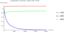
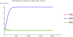
Case 1: w₁ = 3.0, w₂ = 8.5

Equilibrium points:

1) E₁ ≈ (1.1337, 0, 0)

2) E₂ ≈ (1.1337, 0, 0.9)

3) E₃ does not exist (since w₂ > w₂₁ ≈ 0.9)

Eigenvalues at E₂ ≈ (−8.36598, 0.22510, −0.45) - one positive eigenvalue makes E₂ un- stable. The hunting cell population collapses to zero, and the tumor approaches carrying capacity.

Download: Download full-size image

Figure 1. w₁ = 3.0, w₂ = 8.5 - Hunting cells collapse.

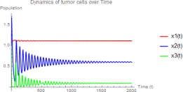
Case 2: w₁ = 3.0, w₂ = 0.8

Here w₂₂ ≈ 0.7364 < w₂ = 0.8 < w₂₁ ≈ 0.9, so E₃ exists and is stable:

E₃ ≈ (1.00690, 0.55776, 0.08182)

The immune system controls but does not eradicate tumor cells, leading to stable coexistence. Initial oscillations dampen as the system approaches equilibrium.

Download: Download full-size image

Figure 2. w₁ = 3.0, w₂ = 0.8 - Stable coexistence equilibrium E₃.

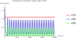
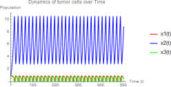
Case 3: w₁ = 3.0, w₂ = 0.5

Since w₂ = 0.5 < w₂₂ ≈ 0.7364, E₃ is unstable, and the system exhibits limit cycle oscillations:

1) Tumor population oscillates around a mean value

2) Hunting cells show large-amplitude oscillations (0.1 to 1.0)

3) Resting cells maintain low-level oscillations

Download: Download full-size image

Figure 3. w₁ = 3.0, w₂ = 0.5 - Unstable E₃ with limit cycle oscillations.

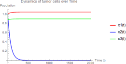
Case 4: w₁ = 0.2, w₂ = 1.0

E₂ is stable:

1) Hunting cells behave like a drug-sensitive clone, eliminated quickly

2) Tumor cells reach near-carrying capacity

3) Resting cells coexist at reduced abundance

Download: Download full-size image

Figure 4. w₁ = 0.2, w₂ = 1.0 - Stable E₂ with hunting cell elimination.

Case 5: w₁ = 0.2, w₂ = 0.8

E₃ is stable, with hunting cells effectively controlling tumor growth:

1) Hunting cells reach system carrying capacity

2) Resting cells persist at low levels

Download: Download full-size image

Figure 5. w₁ = 0.2, w₂ = 0.8 - Stable E₃ with effective immune control.

Case 6: Critical Parameters

At certain parameter values, all equilibria become unstable, leading to sustained regular oscillations:

1) Hunting cells show large amplitude oscillations (2 to 10)

2) Tumor and resting cells oscillate with the same period but smaller amplitude

Download: Download full-size image

Figure 6. All equilibria unstable - Sustained limit cycle oscillations.

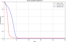
7.2. Numerical Solution of the Optimal Control

We now demonstrate the effectiveness of optimal control for stabilizing unstable equilibria. Using parameter values that yield unstable E₃: a₁ = 6.6, a₂ = 0.5, a₃ = 0.05, a₄ = 0.5, a₅ = 0.6, a₆ = 0.05, w₁ = 0.1, w₂ = 0.7.

The uncontrolled system exhibits oscillations. With optimal controls u₁^∗, u₂^∗, u₃^∗ derived from minimizing cost functional (15), the system stabilizes to equilibrium:

Download: Download full-size image

Figure 7. Controlled system - Optimal controls stabilize the system to equilibrium.

The control inputs initially apply strong therapy to dampen oscillations, then gradually reduce as the system approaches equilibrium. This demonstrates that optimal control theory can successfully design therapeutic interventions to stabilize tumor-immune dynamics

[1, 31]

8. Discussion and Conclusion

This paper presents a mathematical model of tumor-immune interactions that incorporates biologically realistic Holling Type-II functional responses. Unlike previous mass-action model

[10]

, our analysis reveals several novel dynamical features:

1) Multiple equilibria: The model can have none, one, or up to three positive coexistence equilibria, depending on parameter values.

2) Stability transitions: Coexistence equilibria can be stable or unstable, with stability determined by the half-saturation constants w₁ and w₂.

3) Hopf bifurcations: When coexistence equilibria lose stability, the system exhibits sustained limit cycle oscillations, representing periodic fluctuations in all three cell populations

[35]

4) Threshold behavior: The half-saturation constant w₁ has a single threshold value of 1, while w₂ has two thresholds (w₂₁ and w₂₂) that determine system dynamics:

a) w2 > w21: Only E1 and E2 exist

b) w22 < w2 < w21: Stable coexistence E3

c) w2 < w22: Unstable E3 with limit cycles

The optimal control analysis demonstrates that therapeutic interventions can be designed to stabilize unstable equilibria, bringing tumor populations to manageable levels while minimizing treatment costs

[1, 5]

Three important limitations and implications emerge:

First, the oscillatory dynamics predicted by the model, while mathematically interesting, lack empirical support in solid tumors. Further experimental validation is needed

[9]

Second, administering anti-tumor treatments during oscillatory conditions presents clinical challenges. The optimal control framework developed here can guide treatment timing and dosage

[6]

Third, the possibility of multiple tumor equilibrium values for fixed immune cell populations suggests an opportunity to contain cancer at the lowest equilibrium value through appropriate interventions

[19, 23]

Future work should extend this model to include spatial effects, time delays

[2, 7]

, and stochastic elements to capture more complex tumor-immune dynamics. Experimental vali dation of predicted bifurcations and optimal control strategies would strengthen the clinical relevance of this approach.

Conflict of Interest

The authors declare no conflict of interest.

Author contributions

Tewele Assefa Welu: Conceptualization, Formal analysis, Methodology, Software, Writing – original draft

Ataklti Araya: Data curation

Habtu Alemayehu: Supervision, Validation

Yohannes Yirga: Writing – review & editing

Subrata Kumar Sahu: Supervision, Validation

References

[1]	T. Agrawal, M. Saleem, and S. K. Sahu, “Optimal control of the dynamics of a tumor growth model with Hollings type-II functional response,” Computational and Applied Mathematics, vol. 33, no. 3, pp. 591–606, 2014.
[2]	S. Banerjee and R. Sarkar, “Delay-induced model for tumor-immune interaction and con- trol of malignant tumor growth,” Biosystems, vol. 91, pp. 268–288, 2008.
[3]	N. Bellomo, N. Li, and P. Maini, “On the foundations of cancer modeling: selected topics, speculations, and perspectives,” Mathematical Models and Methods in Applied Sciences, vol. 18, no. 4, pp. 593–646, 2008.
[4]	M. Bodnar and U. Forys, “Three types of simple DDE’s describing tumour growth,” Jour- nal of Biological Systems, vol. 15, pp. 1–19, 2007.
[5]	T. Burden, J. Ernstberger, and K. R. Fister, “Optimal control applied to immunotherapy,” Discrete and Continuous Dynamical Systems Series B, vol. 4, no. 1, pp. 135–146, 2004.
[6]	F. Castiglione and B. Piccoli, “Cancer immunotherapy, mathematical modeling and opti- mal control,” Journal of Theoretical Biology, vol. 247, pp. 723–732, 2007.
[7]	A. d’Onofrio, F. Gatti, P. Cerrai, and L. Freschi, “Delay-induced oscillatory dynamics of tumour-immune system interaction,” Mathematical and Computer Modelling, vol. 51, pp. 572–591, 2010.
[8]	L. de Pillis, A. Radunskaya, and C. Wiseman, “A validated mathematical model of cell- mediated immune response to tumor growth,” Cancer Research, vol. 65, no. 17, pp. 7950– 7958, 2005.
[9]	R. Eftimie, J. L. Bramson, and D. J. D. Earn, “Interactions between the immune system and cancer: a brief review of non-spatial mathematical models,” Bulletin of Mathematical Biology, vol. 73, pp. 2–32, 2011.
[10]	A. El-Gohary, “Chaos and optimal control of cancer self-remission and tumor system steady states,” Chaos, Solitons & Fractals, vol. 37, no. 5, pp. 1305–1316, 2008.
[11]	M. Galach, “Dynamics of the tumor-immune system competition - The effect of time delay,” International Journal of Applied Mathematics and Computer Science, vol. 13, no. 3, pp. 395–406, 2003.
[12]	P. Giesl, “Construction of Global Lyapunov functions using Basis functions,” Springer Berlin Heidelberg, New York, 1994.
[13]	B. Goldstein, J. Faeder, and W. Hlavacek, “Mathematical and computational models of immune receptor signaling,” Nature Reviews Immunology, vol. 4, no. 6, pp. 445–456, 2004.
[14]	M. W. Hirsch and S. Smale, “Differential equations, dynamical systems and linear alge- bra,” Academic Press, 1974.
[15]	R. Johnson and M. Patrizia, “Stability and Bifurcation theory for non Autonomous differ- ential equations,” Pera Springer Cetraro, Italy, 2011.
[16]	G. Kaur and N. Ahmad, “A study of population dynamics of normal and malignant cells,”International Journal of Scientific Engineering Research, vol. 4, no. 4, pp. 770–775, 2013.
[17]	D. Kirschner and J. C. Panetta, “Modeling immunotherapy of the tumor-immune interac- tion,” Journal of Mathematical Biology, vol. 37, no. 3, pp. 235–252, 1998.
[18]	N. Kronik, Y. Kogan, V. Vainstein, and Z. Agur, “Improving alloreactive CTL im- munotherapy for malignant gliomas using a simulation model of their interactive dynam- ics,” Cancer Immunology Immunotherapy, vol. 57, pp. 425–439, 2008.
[19]	V. Kuznetsov, I. Makalkin, M. Taylor, and A. Perelson, “Nonlinear dynamics of immuno- genic tumors: parameter estimation and global bifurcation analysis,” Bulletin of Mathe- matical Biology, vol. 56, no. 2, pp. 295–321, 1994.
[20]	M. Martins Jr, S. C. Ferreira, and M. Vilela, “Multiscale models for the growth of avas- cular tumors,” Physics of Life Reviews, vol. 4, pp. 128–156, 2007.
[21]	A. Merola, C. Cosentino, and F. Amato, “An insight into tumor dormancy equilibrium via the analysis of its domain of attraction,” Biomedical Signal Processing and Control, vol. 3, pp. 212–219, 2008.
[22]	W. L. Miranker, “Existence, uniqueness and stability of solution of systems of non linear difference-differential equations,” Journal of Mathematics and Mechanics, vol. 11, no. 1, pp. 101–107, 1962.
[23]	J. D. Murray, “Mathematical Biology,” Springer-Verlag, 1989.
[24]	J. Nagy, “The ecology and evolutionary biology of cancer: a review of mathematical models of necrosis and tumor cells diversity,” Mathematical Biosciences and Engineering, vol. 2, no. 2, pp. 381–418, 2005.
[25]	K. Ogata, “Modern Control Engineering,” Prentice-Hall, Englewood Cliffs, 1970.
[26]	R. Paul, “Stability analysis of critical points to control growth of tumor in an Immune- Tumor-Normal cell-Drug model,” International Journal of Applied Mathematics and Sta- tistical Sciences, vol. 5, pp. 43–52, 2015.
[27]	L. Perko, “Differential Equations and Dynamical Systems,” Springer-Verlag, New York, 2001.
[28]	M. J. Piotrowska, “Hopf bifurcation in a solid avascular tumour growth model with two discrete delays,” Mathematical and Computer Modelling, vol. 47, pp. 597–603, 2008.
[29]	B. Quesnel, “Dormant tumor cells as therapeutic target?” Cancer Letters, vol. 267, pp. 10–17, 2008.
[30]	F. A. Rihan, M. Safan, M. A. Abdeen, and D. Abdel Rahman, “Qualitative and com- putational analysis of a mathematical model for tumor-immune interactions,” Journal of Applied Mathematics, vol. 2012, Article ID 475720, 19 pages, 2012.
[31]	F. A. Rihan, D. H. Abdelrahman, F. Al-Maskari, F. Ibrahim, and M. A. Abdeen, “Delay Differential Model for Tumour-Immune Response with Chemoimmunotherapy and Opti- mal Control,” Computational and Mathematical Methods in Medicine, vol. 2014, Article ID 982978, 2014.
[32]	R. Sachs, L. Hlatky, and P. Hahnfeldt, “Simple ODE models of tumor growth and anti- angiogenic or radiation treatment,” Mathematical and Computer Modelling, vol. 33, pp. 1297–1305, 2001.
[33]	M. Saleem and T. Agrawal, “Chaos in a tumor growth model with delayed responses of the immune system,” Journal of Applied Mathematics, vol. 2012, Article ID 891095, 16 pages, 2012.
[34]	T. H. Stewart, “Immune mechanisms and tumor dormancy,” Medicina (Buenos Aires), vol. 56, no. 1, pp. 74–82, 1996.
[35]	S. H. Strogatz, “Nonlinear Dynamics and Chaos with applications to physics, biology, chemistry, and engineering,” Perseus Books, LLC, Massachusetts, 1994.
[36]	M. D. Vesely, M. H. Kershaw, R. D. Schreiber, and M. J. Smyth, “Natural innate and adaptive immunity to cancer,” Annual Review of Immunology, vol. 29, pp. 235–271, 2011.
[37]	R. A. Weinberg, “The Biology of Cancer,” Garland Sciences, Taylor and Francis, New York, 2007.
[38]	T. L. Whiteside, “Immune suppression in cancer: effects on immune cells, mechanisms and future therapeutic intervention,” Seminars in Cancer Biology, vol. 16, pp. 3–15, 2006.
[39]	B. F. Zamarron and W. J. Chen, “Dual roles of immune cells and their factors in cancer development and progression,” International Journal of Biological Sciences, vol. 7, pp. 651–658, 2011.

Cite This Article

Plain Text BibTeX RIS

APA Style

Welu, T. A., Sahu, S. K., Araya, A., Alemayehu, H., Yirga, Y. (2026). Mathematical Modeling of Tumor-Immune Interaction with Optimal Control in the Human System. Science Discovery Mathematics, 1(1), 34-42. https://doi.org/10.11648/j.sdmath.20260101.14

Copy | Download

ACS Style

Welu, T. A.; Sahu, S. K.; Araya, A.; Alemayehu, H.; Yirga, Y. Mathematical Modeling of Tumor-Immune Interaction with Optimal Control in the Human System. Sci. Discov. Math. 2026, 1(1), 34-42. doi: 10.11648/j.sdmath.20260101.14

Copy | Download

AMA Style

Welu TA, Sahu SK, Araya A, Alemayehu H, Yirga Y. Mathematical Modeling of Tumor-Immune Interaction with Optimal Control in the Human System. Sci Discov Math. 2026;1(1):34-42. doi: 10.11648/j.sdmath.20260101.14

Copy | Download

@article{10.11648/j.sdmath.20260101.14,
  author = {Tewele Assefa Welu and Subrata Kumar Sahu and Ataklti Araya and Habtu Alemayehu and Yohannes Yirga},
  title = {Mathematical Modeling of Tumor-Immune Interaction with Optimal Control in the Human System},
  journal = {Science Discovery Mathematics},
  volume = {1},
  number = {1},
  pages = {34-42},
  doi = {10.11648/j.sdmath.20260101.14},
  url = {https://doi.org/10.11648/j.sdmath.20260101.14},
  eprint = {https://article.sciencepublishinggroup.com/pdf/10.11648.j.sdmath.20260101.14},
  abstract = {This paper presents a mathematical analysis of the immune response to tumor growth, conceptualized through the lens of predator-prey interactions. We investigate a three-dimensional mathematical model that captures the complex dynamics between tumor cells (the prey), hunting immune cells (active predators), and resting immune cells (reservoir population). The model extends classical ecological frameworks to immunology, recognizing that tumors and immune cells engage in a continuous battle for survival within the human body much like species competing in an ecosystem. We first establish the biological validity of our model by proving that all solutions remain positive, exist uniquely, and stay bounded over time essential properties when modeling living systems where negative populations would make no sense. Our analysis reveals that this seemingly simple system harbors surprisingly rich dynamical behavior. Unlike earlier models based on mass-action kinetics, our formulation shows the existence of multiple equilibrium points, representing different disease outcomes: tumor elimination, uncontrolled growth, or chronic persistence. Most notably, we identify conditions under which Hopf bifurcations occur, giving rise to limit cycles periodic oscillations in tumor and immune cell populations that mirror clinical observations of cancer remission and relapse cycles. Recognizing that clinical reality demands more than just understanding these dynamics, we implement a feedback control strategy designed to stabilize tumor populations at clinically manageable levels. Rather than aiming for complete eradication (which may not always be achievable), this approach seeks to transform aggressive growth into a controlled, chronic condition. Numerical simulations demonstrate that our control mechanism can successfully stabilize otherwise unstable equilibria, effectively "taming" the tumor's behavior. Parameter sensitivity analysis reveals that the half-saturation constants play particularly crucial roles in determining system outcomes. These constants, which govern how quickly immune responses saturate with increasing tumor burden, emerge as potential therapeutic targets. The findings suggest that treatments modifying these immunological thresholds might be as important as those directly killing tumor cells a perspective that could inform future immunotherapy strategies. This work bridges ecological modeling, dynamical systems theory, and clinical oncology, offering both theoretical insights into tumor-immune interactions and practical tools for treatment optimization.},
 year = {2026}
}

Copy | Download

TY  - JOUR
T1  - Mathematical Modeling of Tumor-Immune Interaction with Optimal Control in the Human System
AU  - Tewele Assefa Welu
AU  - Subrata Kumar Sahu
AU  - Ataklti Araya
AU  - Habtu Alemayehu
AU  - Yohannes Yirga
Y1  - 2026/03/12
PY  - 2026
N1  - https://doi.org/10.11648/j.sdmath.20260101.14
DO  - 10.11648/j.sdmath.20260101.14
T2  - Science Discovery Mathematics
JF  - Science Discovery Mathematics
JO  - Science Discovery Mathematics
SP  - 34
EP  - 42
PB  - Science Publishing Group
UR  - https://doi.org/10.11648/j.sdmath.20260101.14
AB  - This paper presents a mathematical analysis of the immune response to tumor growth, conceptualized through the lens of predator-prey interactions. We investigate a three-dimensional mathematical model that captures the complex dynamics between tumor cells (the prey), hunting immune cells (active predators), and resting immune cells (reservoir population). The model extends classical ecological frameworks to immunology, recognizing that tumors and immune cells engage in a continuous battle for survival within the human body much like species competing in an ecosystem. We first establish the biological validity of our model by proving that all solutions remain positive, exist uniquely, and stay bounded over time essential properties when modeling living systems where negative populations would make no sense. Our analysis reveals that this seemingly simple system harbors surprisingly rich dynamical behavior. Unlike earlier models based on mass-action kinetics, our formulation shows the existence of multiple equilibrium points, representing different disease outcomes: tumor elimination, uncontrolled growth, or chronic persistence. Most notably, we identify conditions under which Hopf bifurcations occur, giving rise to limit cycles periodic oscillations in tumor and immune cell populations that mirror clinical observations of cancer remission and relapse cycles. Recognizing that clinical reality demands more than just understanding these dynamics, we implement a feedback control strategy designed to stabilize tumor populations at clinically manageable levels. Rather than aiming for complete eradication (which may not always be achievable), this approach seeks to transform aggressive growth into a controlled, chronic condition. Numerical simulations demonstrate that our control mechanism can successfully stabilize otherwise unstable equilibria, effectively "taming" the tumor's behavior. Parameter sensitivity analysis reveals that the half-saturation constants play particularly crucial roles in determining system outcomes. These constants, which govern how quickly immune responses saturate with increasing tumor burden, emerge as potential therapeutic targets. The findings suggest that treatments modifying these immunological thresholds might be as important as those directly killing tumor cells a perspective that could inform future immunotherapy strategies. This work bridges ecological modeling, dynamical systems theory, and clinical oncology, offering both theoretical insights into tumor-immune interactions and practical tools for treatment optimization.
VL  - 1
IS  - 1
ER  -

Copy | Download

Author Information

Tewele Assefa Welu

Faculty of Mathematics & Statistics, Mekelle University, Mekelle, Ethiopia

Contact Email
Subrata Kumar Sahu

Department of Mathematics, ArbaMinch University, Arba Minch, Ethiopia
Ataklti Araya

Faculty of Mathematics & Statistics, Mekelle University, Mekelle, Ethiopia

Contact Email
Habtu Alemayehu

Faculty of Mathematics & Statistics, Mekelle University, Mekelle, Ethiopia

Contact Email
Yohannes Yirga

Faculty of Mathematics & Statistics, Mekelle University, Mekelle, Ethiopia

Contact Email

Download PDF

Submit an Article

Plain Text BibTeX RIS

APA Style

Welu, T. A., Sahu, S. K., Araya, A., Alemayehu, H., Yirga, Y. (2026). Mathematical Modeling of Tumor-Immune Interaction with Optimal Control in the Human System. Science Discovery Mathematics, 1(1), 34-42. https://doi.org/10.11648/j.sdmath.20260101.14

Copy | Download

ACS Style

Welu, T. A.; Sahu, S. K.; Araya, A.; Alemayehu, H.; Yirga, Y. Mathematical Modeling of Tumor-Immune Interaction with Optimal Control in the Human System. Sci. Discov. Math. 2026, 1(1), 34-42. doi: 10.11648/j.sdmath.20260101.14

Copy | Download

AMA Style

Welu TA, Sahu SK, Araya A, Alemayehu H, Yirga Y. Mathematical Modeling of Tumor-Immune Interaction with Optimal Control in the Human System. Sci Discov Math. 2026;1(1):34-42. doi: 10.11648/j.sdmath.20260101.14

Copy | Download

@article{10.11648/j.sdmath.20260101.14,
  author = {Tewele Assefa Welu and Subrata Kumar Sahu and Ataklti Araya and Habtu Alemayehu and Yohannes Yirga},
  title = {Mathematical Modeling of Tumor-Immune Interaction with Optimal Control in the Human System},
  journal = {Science Discovery Mathematics},
  volume = {1},
  number = {1},
  pages = {34-42},
  doi = {10.11648/j.sdmath.20260101.14},
  url = {https://doi.org/10.11648/j.sdmath.20260101.14},
  eprint = {https://article.sciencepublishinggroup.com/pdf/10.11648.j.sdmath.20260101.14},
  abstract = {This paper presents a mathematical analysis of the immune response to tumor growth, conceptualized through the lens of predator-prey interactions. We investigate a three-dimensional mathematical model that captures the complex dynamics between tumor cells (the prey), hunting immune cells (active predators), and resting immune cells (reservoir population). The model extends classical ecological frameworks to immunology, recognizing that tumors and immune cells engage in a continuous battle for survival within the human body much like species competing in an ecosystem. We first establish the biological validity of our model by proving that all solutions remain positive, exist uniquely, and stay bounded over time essential properties when modeling living systems where negative populations would make no sense. Our analysis reveals that this seemingly simple system harbors surprisingly rich dynamical behavior. Unlike earlier models based on mass-action kinetics, our formulation shows the existence of multiple equilibrium points, representing different disease outcomes: tumor elimination, uncontrolled growth, or chronic persistence. Most notably, we identify conditions under which Hopf bifurcations occur, giving rise to limit cycles periodic oscillations in tumor and immune cell populations that mirror clinical observations of cancer remission and relapse cycles. Recognizing that clinical reality demands more than just understanding these dynamics, we implement a feedback control strategy designed to stabilize tumor populations at clinically manageable levels. Rather than aiming for complete eradication (which may not always be achievable), this approach seeks to transform aggressive growth into a controlled, chronic condition. Numerical simulations demonstrate that our control mechanism can successfully stabilize otherwise unstable equilibria, effectively "taming" the tumor's behavior. Parameter sensitivity analysis reveals that the half-saturation constants play particularly crucial roles in determining system outcomes. These constants, which govern how quickly immune responses saturate with increasing tumor burden, emerge as potential therapeutic targets. The findings suggest that treatments modifying these immunological thresholds might be as important as those directly killing tumor cells a perspective that could inform future immunotherapy strategies. This work bridges ecological modeling, dynamical systems theory, and clinical oncology, offering both theoretical insights into tumor-immune interactions and practical tools for treatment optimization.},
 year = {2026}
}

Copy | Download

TY  - JOUR
T1  - Mathematical Modeling of Tumor-Immune Interaction with Optimal Control in the Human System
AU  - Tewele Assefa Welu
AU  - Subrata Kumar Sahu
AU  - Ataklti Araya
AU  - Habtu Alemayehu
AU  - Yohannes Yirga
Y1  - 2026/03/12
PY  - 2026
N1  - https://doi.org/10.11648/j.sdmath.20260101.14
DO  - 10.11648/j.sdmath.20260101.14
T2  - Science Discovery Mathematics
JF  - Science Discovery Mathematics
JO  - Science Discovery Mathematics
SP  - 34
EP  - 42
PB  - Science Publishing Group
UR  - https://doi.org/10.11648/j.sdmath.20260101.14
AB  - This paper presents a mathematical analysis of the immune response to tumor growth, conceptualized through the lens of predator-prey interactions. We investigate a three-dimensional mathematical model that captures the complex dynamics between tumor cells (the prey), hunting immune cells (active predators), and resting immune cells (reservoir population). The model extends classical ecological frameworks to immunology, recognizing that tumors and immune cells engage in a continuous battle for survival within the human body much like species competing in an ecosystem. We first establish the biological validity of our model by proving that all solutions remain positive, exist uniquely, and stay bounded over time essential properties when modeling living systems where negative populations would make no sense. Our analysis reveals that this seemingly simple system harbors surprisingly rich dynamical behavior. Unlike earlier models based on mass-action kinetics, our formulation shows the existence of multiple equilibrium points, representing different disease outcomes: tumor elimination, uncontrolled growth, or chronic persistence. Most notably, we identify conditions under which Hopf bifurcations occur, giving rise to limit cycles periodic oscillations in tumor and immune cell populations that mirror clinical observations of cancer remission and relapse cycles. Recognizing that clinical reality demands more than just understanding these dynamics, we implement a feedback control strategy designed to stabilize tumor populations at clinically manageable levels. Rather than aiming for complete eradication (which may not always be achievable), this approach seeks to transform aggressive growth into a controlled, chronic condition. Numerical simulations demonstrate that our control mechanism can successfully stabilize otherwise unstable equilibria, effectively "taming" the tumor's behavior. Parameter sensitivity analysis reveals that the half-saturation constants play particularly crucial roles in determining system outcomes. These constants, which govern how quickly immune responses saturate with increasing tumor burden, emerge as potential therapeutic targets. The findings suggest that treatments modifying these immunological thresholds might be as important as those directly killing tumor cells a perspective that could inform future immunotherapy strategies. This work bridges ecological modeling, dynamical systems theory, and clinical oncology, offering both theoretical insights into tumor-immune interactions and practical tools for treatment optimization.
VL  - 1
IS  - 1
ER  -

Copy | Download