Abstract
Regression analysis is a core analytical tool widely employed across diverse domains for predicting continuous outcomes, serving as a cornerstone of statistical inference and machine learning applications ranging from economic trend forecasting to healthcare risk assessment and real estate valuation. Choosing an effective regression technique is critical for accurate predictions, yet a daunting challenge for non-experts due to the wide variety of methods, each with distinct assumptions, tuning requirements and applicability boundaries. To address this dilemma, this study conducts a rigorous empirical comparison of five popular regression techniques—Ordinary Least Squares (OLS), Ridge regression, Lasso regression, Elastic Net, and Polynomial regression—applied to house price prediction using two benchmark datasets: the classic Boston Housing dataset and the comprehensive California Housing dataset. A multi-dimensional evaluation framework was adopted, including quantitative metrics (Mean Squared Error (MSE) and coefficient of determination () and qualitative diagnostics (residual analysis and Quantile-Quantile (QQ) plots) to assess prediction accuracy and error distribution. Results indicate that Polynomial regression consistently achieves superior performance across both datasets, highlighting its effectiveness in capturing the complex nonlinear relationships inherent in housing data. Ridge, Lasso, and Elastic Net provide comparable but lower performance, with strengths in mitigating multicollinearity rather than enhancing nonlinear fitting. OLS yields acceptable baseline results but less robust performance when confronted with real-world nonlinearities. These findings offer clear practical guidance for non-experts seeking reliable “out-of-the-box” regression techniques, and contribute valuable insights to assist practitioners in model selection for real-world predictive tasks without extensive tuning.
Keywords
Regression Analysis, House Price Prediction, Polynomial Regression, Ridge Regression, Model Comparison
1. Introduction
Regression analysis is a fundamental and widely used technique in statistics and machine learning, essential for modeling relationships between dependent and independent variables to make predictions, infer causal effects, or identify underlying patterns
| [1] | Hastie, T., Tibshirani, R. & Friedman, J. The Elements of Statistical Learning: Data Mining, Inference, and Prediction. (Springer, 2009). |
| [2] | James, G., Witten, D., Hastie, T. & Tibshirani, R. An Introduction to Statistical Learning. (Springer, 2013). |
[1, 2]
. Its versatility has led to extensive applications across diverse fields such as economics, finance, healthcare, environmental science, engineering, social sciences, and real estate
| [3] | Kuhn, M. & Johnson, K. Applied Predictive Modeling. (Springer, 2013). |
| [4] | Goodfellow, I., Bengio, Y., & Courville, A. Deep Learning. (MIT Press, 2016). |
| [5] | Breiman, L. Random forests. Mach. Learn. 45, 5-32 (2001). https://doi.org/10.1023/A:1010933404324 |
[3-5]
.
In economics and finance, regression models help forecast market trends, asset prices, and economic indicators. For example, financial analysts use regression techniques to predict stock prices or assess risk factors impacting investment portfolios
| [6] | Glaeser, E. L., Gyourko, J. & Saks R. E. Why is Manhattan so expensive? Regulation and the rise in housing prices. J. Law Econ. 48, 331-373 (2005). |
[6]
. In healthcare, regression aids in understanding the influence of patient characteristics on health outcomes, such as disease progression or treatment efficiency
| [7] | Mora-Garcia, R. T., Cespedes-Lopez, M. F., Perez-Sanchez, V. R. Housing price prediction using machine learning algorithms in COVID-19 times. Land 11, 2100 (2022).
https://doi.org/10.3390/land11112100 |
[7]
. Environmental scientists apply regression to analyze pollution effects on climate change or biodiversity
| [8] | Soltani, A., Heydari, M., Aghaei, F., Pettit, C. J. Housing price prediction incorporating spatio-temporal dependency into machine learning algorithms. Cities 131:103941 (2022).
https://doi.org/10.1016/j.cities.2022.103941 |
[8]
. Similarly, in engineering, regression models support quality control and reliability analysis by predicting failure rates or system performance
.
The classical approach to regression is Ordinary Least Squares (OLS) linear regression, which estimates the relationship assuming linearity between inputs and outputs
1. However, real-world data often violate these assumptions due to multicollinearity, nonlinear relationships, noise, outliers, or high-dimensionality
| [10] | Friedman, J., Hastie, T., Tibshirani, R. Regularization paths for generalized linear models via coordinate descent. J. Stat. Softw. 33, 1-22 (2010).
https://doi.org/10.18637/jss.v033.i01 |
[10]
. To address these issues, researchers have developed more advanced methods such as Ridge regression (which adds an L2 penalty to reduce coefficient variance and combat multicollinearity)
| [10] | Friedman, J., Hastie, T., Tibshirani, R. Regularization paths for generalized linear models via coordinate descent. J. Stat. Softw. 33, 1-22 (2010).
https://doi.org/10.18637/jss.v033.i01 |
[10]
, Lasso regression that includes an L1 penalty promoting sparsity and feature selection
, and Elastic Net, a hybrid combining L1 and L2 penalties to balance shrinkage and sparsity while handling correlated predictors effectively
.
Moreover, to capture nonlinear dependencies in data while maintaining interpretability, Polynomial regression expands the input space using polynomial basis functions
| [1] | Hastie, T., Tibshirani, R. & Friedman, J. The Elements of Statistical Learning: Data Mining, Inference, and Prediction. (Springer, 2009). |
| [2] | James, G., Witten, D., Hastie, T. & Tibshirani, R. An Introduction to Statistical Learning. (Springer, 2013). |
[1, 2]
. This method retains linearity with respect to model parameters but allows modeling of nonlinear patterns inherent in complex datasets.
Despite the availability of these powerful tools, practitioners often face challenges when choosing the most appropriate regression technique for their specific problem. This challenge is compounded for non-expert users who may lack deep statistical or computational expertise. Such users frequently rely on simple linear models due to their interpretability and ease of use but may suffer from suboptimal predictive performance if nonlinearities or feature interactions are present
| [13] | Sharma, S., Arora, D., Shankar, G., & Sharma, P. House Price Prediction Using Machine Learning Algorithm. IEEE ICCMC Conf., pp 982-986 (2023).
https://doi.org/10.1109/ICCMC56507.2023.10084197 |
| [14] | Cellmer, R., Kobylińska, K., Housing price prediction-machine learning and geostatistical methods. Real Estate Manag Valuat 33(1), 1-10 (2025).
https://doi.org/10.2478/remav-2025-0001 |
[13, 14]
.
Relatively few studies have explicitly addressed the practical usability of regression methods for non-specialists. Most research focuses on developing new algorithms or improving benchmarks rather than providing clear guidance on method selection for typical users
| [15] | Hoxha, V. Comparative analysis of machine learning models in predicting housing prices: A case study of Prishtina’s real estate market. Int J Hous Mark Anal 18(3), 694-711 (2023). https://doi.org/10.1108/IJHMA-09-2023-0120 |
[15]
. Existing comparative studies often evaluate methods on synthetic datasets or narrowly defined problems, limiting their generalizability to diverse real-world scenarios
| [16] | Pace, R. K., Barry, R. & Sirmans, C. F. Spatial statistics and real estate. J. Real Estate Finance Econ. 17, 5-13 (1998). |
[16]
.
Some empirical comparisons have been conducted using benchmark datasets like housing price prediction, a canonical task involving heterogeneous features with nonlinear interactions. These studies generally report metrics such as Mean Squared Error (MSE) or R-squared but often lack in-depth residual diagnostics or visualization analyses that could reveal nuanced model behaviors
| [17] | Akaike, H. A new look at the statistical model identification. IEEE Trans Autom Control 19(6), 716-723 (1974).
http://dx.doi.org/10.1109/TAC.1974.1100705 |
| [18] | Breiman, L., Friedman, J. H., Olshen, R. A., Stone, C. J., Classification and Regression Trees. (Wadsworth, 1984). |
[17, 18].
The housing price context has been widely studied in spatial statistics and real estate finance as well
| [19] | Harrison, D. Jr., Rubinfeld, D. L. Hedonic housing prices and the demand for clean air. J Environ Econ Manag 5(1), 81-102 (1978). https://doi.org/10.1016/0095-0696(78)90006-2 |
| [20] | Pedregosa, F., et al. Scikit-learn: Machine learning in Python. J Mach Learn Res 12, 2825-2830 (2011). |
[19, 20]
.
Visualization tools like Quantile-Quantile (QQ) plots are valuable yet underutilized in assessing how well residuals conform to assumptions such as normality—a critical aspect for validating model inference reliability
| [2] | James, G., Witten, D., Hastie, T. & Tibshirani, R. An Introduction to Statistical Learning. (Springer, 2013). |
[2]
.
Automated machine learning (AutoML) frameworks have emerged to assist non-experts by automating model selection and tuning processes
. While promising, AutoML systems tend to be computationally intensive and sometimes opaque regarding rationale behind chosen models, potentially reducing user trust and interpretability.
In practice, simpler models such as OLS are favored for their transparency but may fail to capture important data complexities. Conversely, methods like polynomial regression or regularized models can improve accuracy but require some parameter tuning and understanding of their mechanisms
. Advanced machine learning methods such as random forests and gradient boosting have been proposed for similar tasks but often at the cost of interpretability
.
This gap highlights the need for comprehensive empirical evaluations comparing popular regression techniques on representative real-world datasets using both quantitative metrics and visual diagnostic methods. Such analyses can empower non-expert users to make informed decisions about selecting effective “out-of-the-box” regression solutions for common tasks like house price prediction.
Our study contributes to addressing this need by systematically comparing five widely used regression methods—OLS, Ridge, Lasso, Elastic Net, and Polynomial regression—on two benchmark housing datasets
| [19] | Harrison, D. Jr., Rubinfeld, D. L. Hedonic housing prices and the demand for clean air. J Environ Econ Manag 5(1), 81-102 (1978). https://doi.org/10.1016/0095-0696(78)90006-2 |
| [20] | Pedregosa, F., et al. Scikit-learn: Machine learning in Python. J Mach Learn Res 12, 2825-2830 (2011). |
[19, 20]
. By combining performance metrics with residual and QQ plot analyses, we provide practical recommendations that facilitate reliable model choice without requiring extensive expertise or complex tuning.
2. Methods
To conduct this study, we designed a systematic approach that begins with a comprehensive review of several widely used regression techniques. This review provides a foundation for understanding the principles and differences among these methods. Following this, we introduce a visualization tool known as the Quantile-Quantile (QQ) plot, which plays a crucial role in evaluating the distributional properties of regression residuals and assessing model fit beyond standard numerical metrics.
Our methodology then involves applying each selected regression technique to carefully chosen representative datasets related to house price prediction. These datasets serve as practical test cases to examine how each method performs in real-world scenarios. Through rigorous experimentation, we analyze the predictive accuracy and residual behavior of each model.
Finally, we synthesize the quantitative results and visual analyses to draw meaningful conclusions about the strengths and limitations of each regression approach. This structured process aims to provide clear, actionable insights for users seeking effective “out-of-the-box” regression solutions. The following sections detail the regression techniques under study, the visualization methods employed, the datasets used, and the experimental procedures followed.
2.1. Review of Regression Techniques
Regression analysis is a classical and essential topic in statistics and machine learning, with a wide variety of techniques available to address different data characteristics and modeling needs. For practitioners, especially those new to the field, selecting an appropriate regression method can be challenging given the extensive range of options. To provide focused guidance, this study concentrates on five widely used regression techniques: Ordinary Least Squares (OLS), Ridge regression, Lasso regression, Elastic Net, and Polynomial regression. We briefly review their key principles before applying them to representative datasets for performance evaluation.
2.1.1. Ordinary Least Squares
Ordinary Least Squares (OLS) is a foundational technique in linear regression, serving as a baseline method for modeling the relationship between a set of independent variables and a continuous target variable. OLS estimates the regression coefficients by minimizing the residual sum of squares (RSS) between the observed target values and the predicted values , where denotes the feature matrix and represents the coefficient vector. Formally, the optimization problem is defined as:
Under the classical assumptions of linear regression—linearity, independence, homoscedasticity, and normally distributed errors—OLS provides the Best Linear Unbiased Estimators (BLUE). This method is particularly effective when multicollinearity is not present and when the number of observations exceeds the number of features.
2.1.2. Ridge Regression
Ridge regression, also known as Tikhonov regularization, extends the OLS framework by incorporating a regularization term that penalizes large coefficients. This is particularly advantageous in scenarios involving multicollinearity or when the feature space is high-dimensional. The ridge regression objective function is given by:
Here, is a regularization hyperparameter that controls the degree of shrinkage applied to the coefficients. As increases, the model becomes more conservative, yielding smaller coefficient magnitudes and enhancing generalization at the potential cost of increased bias. Ridge regression retains all features but shrinks their coefficients, thereby mitigating the effects of multicollinearity and reducing model variance.
2.1.3. Lasso Regression
The Least Absolute Shrinkage and Selection Operator (Lasso) regression modifies the OLS objective by introducing an -norm penalty on the regression coefficients, promoting sparsity in the solution. This property makes Lasso particularly suitable for feature selection in high-dimensional datasets. The objective function is expressed as:
(3)
where denotes the -norm of the coefficient vector and is a tuning parameter controlling the strength of the regularization. The Lasso tends to produce models that involve only a subset of the input features, as it can drive some coefficients exactly to zero. This sparsity-inducing behavior has led to its widespread use in the context of compressed sensing and high-dimensional statistical modeling. In practice, coordinate descent is a commonly employed algorithm for solving the Lasso optimization problem.
2.1.4. Elastic-Net
Elastic Net regression combines the penalties of both Lasso (-norm) and Ridge (-norm) regularizations, offering a compromise between sparsity and coefficient shrinkage. The model is particularly useful when dealing with groups of correlated variables, where Lasso may arbitrarily select one feature from the group, while Elastic Net tends to retain multiple correlated predictors. The objective function for Elastic Net is defined as:
(4)
Here, governs the overall strength of the regularization, and controls the balance between the and penalties. When , the model reduces to Lasso; when , it simplifies to Ridge regression. Elastic Net thus inherits the variable selection capability of Lasso and the stability properties of Ridge, making it a robust choice in a wide range of regression settings, particularly when predictors exhibit high collinearity.
2.1.5. Polynomial Regression: Extending Linear Models with Basis Functions
Polynomial regression extends the classical linear regression framework by incorporating nonlinear transformations of the original input features through the use of polynomial basis functions. Despite the nonlinear relationship introduced between the transformed features and the original inputs, the model retains its linearity with respect to the coefficients, thereby allowing the use of standard linear regression techniques for estimation.
In the canonical form of linear regression for a two-dimensional feature vector , the model is expressed as:
To enable the model to capture quadratic interactions and nonlinear trends, the input space can be expanded using second-degree polynomial basis functions. The resulting model takes the form:
(6)
This formulation can be interpreted as a linear regression model applied to an augmented feature space defined by:
Accordingly, the model can be rewritten as:
(8)
This illustrates that polynomial regression remains a member of the linear model family, as it is linear with respect to the coefficient vector . The transformation of the input data through polynomial basis functions allows for greater model flexibility, enabling the capture of nonlinear dependencies in the data while preserving the interpretability and computational advantages of linear regression.
Polynomial regression is particularly useful when prior knowledge or exploratory analysis suggests the presence of nonlinear patterns, yet a fully nonlinear model may not be justified or desirable. The degree of the polynomial can be adjusted to balance model complexity and generalization, and regularization methods such as Ridge, Lasso, or Elastic Net can be incorporated to mitigate overfitting in high-degree expansions.
2.1.6. Visualization Techniques: Quantile-Quantile (QQ) Plot
The Quantile-Quantile (QQ) plot is a diagnostic graphical technique employed to evaluate the degree of correspondence between the empirical distribution of a dataset and a specified theoretical distribution, most commonly the normal distribution. It is a widely used method for assessing distributional assumptions in statistical modeling and inference.
In a QQ plot, the theoretical quantiles of the reference distribution are plotted along the horizontal axis, while the corresponding sample quantiles derived from the observed data are plotted along the vertical axis. If the empirical data follow the theoretical distribution closely, the plotted points will align approximately along the reference line, typically the 45-degree line passing through the origin.
Departures from this diagonal pattern provide insight into distributional deviations. For instance, systematic curvature may indicate skewness, while deviations in the tails may suggest heavy-tailed behavior or the presence of outliers. Consequently, the QQ plot serves as a valuable tool for detecting violations of normality, identifying data irregularities, and guiding model selection and transformation strategies.
QQ plots are extensively utilized in various domains, including finance, engineering, biomedical sciences, and social sciences, particularly in contexts involving hypothesis testing, model diagnostics, and validation of parametric assumptions. Due to their interpretability and general applicability, QQ plots are considered an essential component of the statistical visualization toolkit.
2.1.7. Datasets Employed in Empirical Evaluation
To facilitate a representative exploration of regression techniques, this study focuses on the well-established task of housing price prediction. Housing datasets offer rich, heterogeneous feature spaces and real-world relevance, making them particularly suitable for evaluating the performance and interpretability of regression models.
In this work, two widely recognized benchmark datasets are utilized. Both have been extensively employed in the literature as standard references for algorithm comparison and methodological demonstrations.
3. Experimental Setup
3.1. Boston Housing Dataset
The Boston Housing dataset is a classic regression benchmark that predicts the median value of owner-occupied homes in various suburbs of Boston, Massachusetts. It comprises 506 samples with 13 numerical features capturing socioeconomic and environmental attributes, such as, CRIM: Per capita crime rate by town; RM: Average number of rooms per dwelling; AGE: Proportion of owner-occupied units built prior to 1940 etc. The target variable is the median home value (in thousands of U.S. dollars). This dataset is freely available on many mainstream dataset-sharing websites and has been widely used to illustrate linear modeling techniques and assess predictive performance.
3.2. California Housing Dataset
The California Housing dataset extends the housing price prediction task to a larger and more contemporary context. It includes data on housing across California districts, with 20,640 observations and 8 features that describe geographic, demographic, and economic factors. Key features include MedInc: Median income in the block; HouseAge: Median age of housing units; AveRooms: Average number of rooms per household; Population: Total population of the district etc. The target variable is the median house value for each district. This dataset is also publicly available through many mainstream dataset-sharing websites and is frequently used in machine learning tasks involving large-scale, real-world data.
Together, these datasets offer complementary challenges in terms of feature diversity, scale, and underlying data distributions, thereby enabling a robust and comparative assessment of regression methodologies.
3.3. Hardware and Software Environment
All experiments in this study were conducted using Python, leveraging the widely adopted Scikit-Learn machine learning library for model development and evaluation. The computational environment consisted of a personal computer equipped with an Intel(R) Core(TM) i7-10750H CPU @ 2.60GHz and 32 GB RAM, providing sufficient resources for training and testing on both datasets.
3.4. Implementation Details and Parameter Configuration
Five regression techniques were applied to the selected datasets: Ordinary Least Squares (OLS), Ridge Regression, Lasso Regression, Elastic Net, and Polynomial Regression. For each method, we utilized the corresponding implementations provided by the Scikit-Learn library, adhering to default algorithmic configurations unless otherwise specified.
The datasets were partitioned into training and testing sets using an 80:20 split—a conventional choice in machine learning practice that balances training sufficiency with evaluation reliability.
The regularization parameters were configured as follows:
1) Ridge Regression: Regularization strength
2) Lasso Regression: Regularization strength
3) Elastic Net: Regularization strength , and mixing parameter
Polynomial regression was performed with second-degree polynomial feature expansion to allow the model to capture nonlinear relationships without deviating from the linear modeling framework.
4. Results and Discussion
4.1. Boston Housing Dataset: Model Performance Evaluation
This section presents the predictive performance of the selected regression models on the Boston Housing dataset. Each model was trained using the specified parameter configurations and evaluated on the held-out test set.
Table 1 summarizes the predictive performance of the five regression models in terms of Mean Squared Error (MSE) and R-squared (
). Among the models evaluated, Polynomial Regression outperformed all others, achieving the lowest MSE of 14.18 and the highest
score of 0.81. This indicates a significantly better fit to the data, likely due to the model's ability to capture nonlinear relationships via second-degree polynomial feature expansion. In contrast, the remaining four models—Linear Regression, Ridge, Lasso, and Elastic Net—exhibited comparable performance, all yielding an
value of approximately 0.67, with minor variations in MSE. This suggests that while regularization slightly affects the numerical stability of the coefficients, it does not substantially enhance predictive performance in this particular dataset, possibly due to the moderate dimensionality and absence of severe multicollinearity. The results affirm the advantage of incorporating nonlinear feature transformations when the underlying data-generating process exhibits nonlinearity.
Table 1. Performance of five regression techniques on the Boston Housing dataset.
Method | Mean Squared Error (MSE) | R-squared () |
OLS | 24.29 | 0.67 |
Ridge | 24.48 | 0.67 |
Lasso | 24.41 | 0.67 |
Elastic Net | 23.97 | 0.67 |
Polynomial | 14.18 | 0.81 |
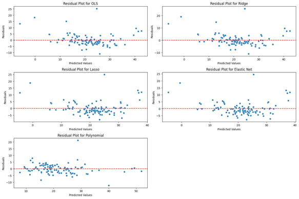
Figure 1 displays the residual plots corresponding to the five regression models evaluated: Ordinary Least Squares (OLS), Ridge, Lasso, Elastic Net, and Polynomial Regression. Residual plots are a diagnostic tool used to assess model performance by visualizing the distribution of prediction errors—i.e., the differences between observed and predicted values. Among the models, Polynomial Regression exhibits the most favorable residual behavior. The residuals are not only tightly clustered around the zero-reference line but also fall within a relatively narrow range, suggesting both low variance and minimal bias. This aligns with the previously observed superior performance in terms of Mean Squared Error (MSE) and
. While Ridge Regression also demonstrates a relatively narrow spread in its residuals, the distribution is more dispersed compared to Polynomial Regression. Additionally, the Ridge residuals exhibit mild systematic deviation from the zero line, suggesting minor model underfitting or inability to fully capture nonlinearity. By contrast, the residuals from OLS, Lasso, and Elastic Net show larger deviations and less consistent alignment around the zero axis, indicating greater error variance and reduced predictive fidelity. These patterns reinforce the conclusion that introducing nonlinear basis functions via polynomial expansion significantly enhances model fit for this dataset.
Figure 1. Residual plots for the five regression techniques applied to the Boston Housing dataset.
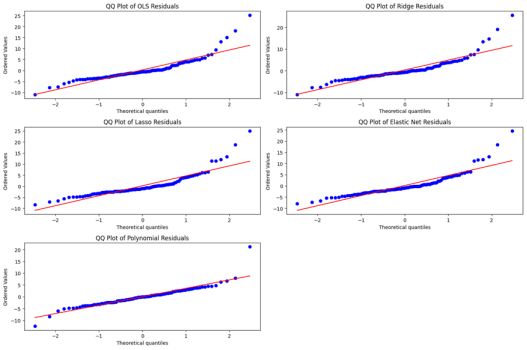
Figure 2 presents the Quantile-Quantile (QQ) plots for the residuals of each regression technique applied to the Boston Housing dataset. These plots are used to assess the extent to which residuals conform to a normal distribution, which is a key assumption in many regression-based inference procedures. In a QQ plot, theoretical quantiles from the normal distribution are plotted on the x-axis, while the ordered sample residuals are plotted on the y-axis. A well-fitting model will yield residuals that align closely with the reference line (in red), indicating approximate normality. Among the five models, Polynomial Regression exhibits the most favorable QQ plot. The residuals are closely aligned with the diagonal line, especially across the central quantiles, indicating that the error distribution closely follows a Gaussian pattern. This further reinforces the model’s strong predictive performance, as seen in the previous residual and performance metrics analysis. By contrast, the residuals from OLS, Ridge, Lasso, and Elastic Net exhibit noticeable deviations from normality, particularly in the tails. These deviations suggest the presence of skewness and heavy-tailed behavior, which may affect the validity of statistical inferences based on these models.
Figure 2. Quantile-Quantile (QQ) plots of residuals for the five regression models.
4.2. California Housing Dataset: Model Performance Evaluation
This section presents the predictive performance of the selected regression models on the California Housing dataset. As shown in
Table 2, Polynomial Regression once again outperforms the other methods, achieving the lowest MSE and the highest
value. The improvement in
from 0.58 to 0.66 indicates a more accurate fit and better generalization to unseen data. The other four models—Linear, Ridge, Lasso, and Elastic Net—exhibit nearly identical performance, with Ridge and Lasso showing negligible differences from the baseline linear model. These results suggest that incorporating polynomial basis functions enables the model to capture nonlinear relationships present in the California housing data, leading to improved predictive performance.
Table 2. Performance of five regression techniques on the California Housing dataset.
Method | Mean Squared Error (MSE) | R-squared () |
OLS | 5.81E+09 | 0.58 |
Ridge | 5.81E+09 | 0.58 |
Lasso | 5.81E+09 | 0.58 |
Elastic Net | 5.99E+09 | 0.56 |
Polynomial | 4.61E+09 | 0.66 |
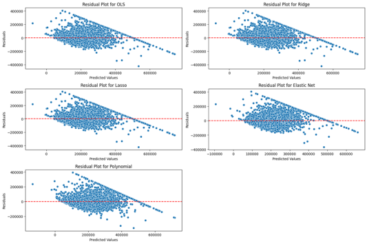
Figure 3 presents the residual plots corresponding to each regression model. Consistent with the results observed for the Boston dataset, the residuals from Polynomial Regression are more symmetrically distributed around the zero baseline and exhibit reduced variance compared to the other models. In contrast, the residuals from OLS, Ridge, Lasso, and Elastic Net demonstrate a distinct triangular pattern, with prediction errors increasing in magnitude alongside the predicted values. This heteroscedastic behavior suggests that these models may fail to capture underlying nonlinearities or complex interactions among features.
Figure 3. Residual plots for the five regression models applied to the California Housing dataset.
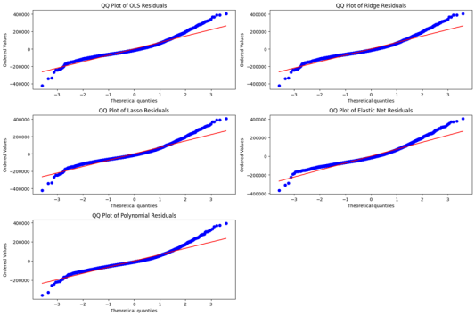
Figure 4 displays the QQ plots of residuals, providing insight into the normality assumption. As with the Boston Housing dataset, Polynomial Regression demonstrates residuals most closely aligned with the diagonal line, particularly in the central quantiles. This indicates a closer adherence to normality and fewer extreme deviations. The residuals from the other models exhibit noticeable departures from the reference line, particularly in the tails, indicating heavier-tailed distributions and potential issues with skewness. These deviations can negatively impact inference tasks that rely on the assumption of normally distributed errors.
Figure 4. QQ plots of residuals for the five regression models applied to the California Housing dataset.
Together, the residual and QQ plot analyses further corroborate the quantitative results, confirming that Polynomial Regression is the most suitable model for the California housing price prediction task among those evaluated. It not only reduces prediction error but also produces more normally distributed and homoscedastic residuals, making it a robust choice in the presence of nonlinear patterns in the data.
5. Conclusions
This study addressed a core practical problem: identifying the optimal regression technique for non-expert users to achieve reliable predictive performance on typical continuous outcome tasks using only default model settings, without specialized tuning or domain expertise. We empirically compared five common methods—Ordinary Least Squares (OLS), Ridge, Lasso, Elastic Net, and Polynomial Regression—on the Boston and California Housing datasets, with evaluations spanning quantitative metrics (MSE, ) and qualitative diagnostics (residuals, QQ plots).
Key findings show that Polynomial Regression with second-degree features consistently outperforms the other four methods in both predictive accuracy and residual conformity, effectively capturing the nonlinear relationships inherent in housing data without complex adjustments. Linear regularization models (Ridge, Lasso, Elastic Net) delivered comparable but lower performance, while OLS yielded acceptable but less robust baseline results.
These findings confirm Polynomial Regression as a practical, accessible choice for non-experts tackling general regression tasks. Future research directions can include testing these methods on datasets with stronger feature collinearity and exploring automated nonlinear feature engineering to further boost the performance of out-of-the-box regression solutions. Overall, this work provides valuable guidance for practitioners seeking reliable, low-threshold predictive tools.
Abbreviations
OLS | Ordinary Least Squares |
MSE | Mean Squared Error |
QQ Plot | Quantile-Quantile Plot |
AutoML | Automated Machine Learning |
RSS | Residual Sum of Squares |
Author Contributions
Jie Wang: Conceptualization, Methodology, Writing – original draft
Qiutong Yu: Data curation, Investigation, Visualization
Xintong Liu: Data curation, Investigation, Visualization
Hongli Zhu: Data curation, Investigation, Visualization
Qiuyu Ming: Data curation, Investigation, Visualization
Jiatong Dai: Data curation, Investigation, Visualization
Guanyu Sha: Data curation, Investigation, Visualization
Hanyu Xu: Data curation, Investigation, Visualization
Yan Zhong: Data curation, Investigation, Visualization
Shancheng Yu: Project administration, Investigation, Writing – review & editing
Conflicts of Interest
The authors declare no competing interests.
References
| [1] |
Hastie, T., Tibshirani, R. & Friedman, J. The Elements of Statistical Learning: Data Mining, Inference, and Prediction. (Springer, 2009).
|
| [2] |
James, G., Witten, D., Hastie, T. & Tibshirani, R. An Introduction to Statistical Learning. (Springer, 2013).
|
| [3] |
Kuhn, M. & Johnson, K. Applied Predictive Modeling. (Springer, 2013).
|
| [4] |
Goodfellow, I., Bengio, Y., & Courville, A. Deep Learning. (MIT Press, 2016).
|
| [5] |
Breiman, L. Random forests. Mach. Learn. 45, 5-32 (2001).
https://doi.org/10.1023/A:1010933404324
|
| [6] |
Glaeser, E. L., Gyourko, J. & Saks R. E. Why is Manhattan so expensive? Regulation and the rise in housing prices. J. Law Econ. 48, 331-373 (2005).
|
| [7] |
Mora-Garcia, R. T., Cespedes-Lopez, M. F., Perez-Sanchez, V. R. Housing price prediction using machine learning algorithms in COVID-19 times. Land 11, 2100 (2022).
https://doi.org/10.3390/land11112100
|
| [8] |
Soltani, A., Heydari, M., Aghaei, F., Pettit, C. J. Housing price prediction incorporating spatio-temporal dependency into machine learning algorithms. Cities 131:103941 (2022).
https://doi.org/10.1016/j.cities.2022.103941
|
| [9] |
Wold, S., Sjöström, M., Eriksson, L. PLS-regression: A basic tool of chemometrics. Chemom. Intell. Lab. Syst. 58, 109-130 (2001).
https://doi.org/10.1016/S0169-7439(01)00155-1
|
| [10] |
Friedman, J., Hastie, T., Tibshirani, R. Regularization paths for generalized linear models via coordinate descent. J. Stat. Softw. 33, 1-22 (2010).
https://doi.org/10.18637/jss.v033.i01
|
| [11] |
Tibshirani, R. Regression shrinkage and selection via the lasso. J. R. Stat. Soc. Ser. B 58, 267-288 (1996).
https://doi.org/10.1111/j.2517-6161.1996.tb02080.x
|
| [12] |
Zou, H., Hastie, T. Regularization and variable selection via the elastic net. J. R. Stat. Soc. Ser. B 67, 301–320 (2005).
https://doi.org/10.1111/j.1467-9868.2005.00503.x
|
| [13] |
Sharma, S., Arora, D., Shankar, G., & Sharma, P. House Price Prediction Using Machine Learning Algorithm. IEEE ICCMC Conf., pp 982-986 (2023).
https://doi.org/10.1109/ICCMC56507.2023.10084197
|
| [14] |
Cellmer, R., Kobylińska, K., Housing price prediction-machine learning and geostatistical methods. Real Estate Manag Valuat 33(1), 1-10 (2025).
https://doi.org/10.2478/remav-2025-0001
|
| [15] |
Hoxha, V. Comparative analysis of machine learning models in predicting housing prices: A case study of Prishtina’s real estate market. Int J Hous Mark Anal 18(3), 694-711 (2023).
https://doi.org/10.1108/IJHMA-09-2023-0120
|
| [16] |
Pace, R. K., Barry, R. & Sirmans, C. F. Spatial statistics and real estate. J. Real Estate Finance Econ. 17, 5-13 (1998).
|
| [17] |
Akaike, H. A new look at the statistical model identification. IEEE Trans Autom Control 19(6), 716-723 (1974).
http://dx.doi.org/10.1109/TAC.1974.1100705
|
| [18] |
Breiman, L., Friedman, J. H., Olshen, R. A., Stone, C. J., Classification and Regression Trees. (Wadsworth, 1984).
|
| [19] |
Harrison, D. Jr., Rubinfeld, D. L. Hedonic housing prices and the demand for clean air. J Environ Econ Manag 5(1), 81-102 (1978).
https://doi.org/10.1016/0095-0696(78)90006-2
|
| [20] |
Pedregosa, F., et al. Scikit-learn: Machine learning in Python. J Mach Learn Res 12, 2825-2830 (2011).
|
| [21] |
Chen, T., Guestrin, C. XGBoost: A scalable tree boosting system. In Proc 22nd ACM SIGKDD Int Conf Knowl Discov Data Min. pp 785-794 (2016).
https://doi.org/10.1145/2939672.2939785
|
Cite This Article
-
APA Style
Wang, J., Yu, Q., Liu, X., Zhu, H., Ming, Q., et al. (2026). Unveiling the Impact of Nonlinear Modeling in Housing Price Prediction: An Empirical Comparative Study. Science Journal of Applied Mathematics and Statistics, 14(1), 6-15. https://doi.org/10.11648/j.sjams.20261401.12
 Copy
|
Copy
|
 Download
ACS Style
Wang, J.; Yu, Q.; Liu, X.; Zhu, H.; Ming, Q., et al. Unveiling the Impact of Nonlinear Modeling in Housing Price Prediction: An Empirical Comparative Study. Sci. J. Appl. Math. Stat. 2026, 14(1), 6-15. doi: 10.11648/j.sjams.20261401.12
Copy
|
Download
AMA Style
Wang J, Yu Q, Liu X, Zhu H, Ming Q, et al. Unveiling the Impact of Nonlinear Modeling in Housing Price Prediction: An Empirical Comparative Study. Sci J Appl Math Stat. 2026;14(1):6-15. doi: 10.11648/j.sjams.20261401.12
Copy
|
Download
-
@article{10.11648/j.sjams.20261401.12,
  author = {Jie Wang and Qiutong Yu and Xintong Liu and Hongli Zhu and Qiuyu Ming and Jiatong Dai and Guanyu Sha and Hanyu Xu and Yan Zhong and Shancheng Yu},
  title = {Unveiling the Impact of Nonlinear Modeling in Housing Price Prediction: An Empirical Comparative Study},
  journal = {Science Journal of Applied Mathematics and Statistics},
  volume = {14},
  number = {1},
  pages = {6-15},
  doi = {10.11648/j.sjams.20261401.12},
  url = {https://doi.org/10.11648/j.sjams.20261401.12},
  eprint = {https://article.sciencepublishinggroup.com/pdf/10.11648.j.sjams.20261401.12},
  abstract = {Regression analysis is a core analytical tool widely employed across diverse domains for predicting continuous outcomes, serving as a cornerstone of statistical inference and machine learning applications ranging from economic trend forecasting to healthcare risk assessment and real estate valuation. Choosing an effective regression technique is critical for accurate predictions, yet a daunting challenge for non-experts due to the wide variety of methods, each with distinct assumptions, tuning requirements and applicability boundaries. To address this dilemma, this study conducts a rigorous empirical comparison of five popular regression techniques—Ordinary Least Squares (OLS), Ridge regression, Lasso regression, Elastic Net, and Polynomial regression—applied to house price prediction using two benchmark datasets: the classic Boston Housing dataset and the comprehensive California Housing dataset. A multi-dimensional evaluation framework was adopted, including quantitative metrics (Mean Squared Error (MSE) and coefficient of determination () and qualitative diagnostics (residual analysis and Quantile-Quantile (QQ) plots) to assess prediction accuracy and error distribution. Results indicate that Polynomial regression consistently achieves superior performance across both datasets, highlighting its effectiveness in capturing the complex nonlinear relationships inherent in housing data. Ridge, Lasso, and Elastic Net provide comparable but lower performance, with strengths in mitigating multicollinearity rather than enhancing nonlinear fitting. OLS yields acceptable baseline results but less robust performance when confronted with real-world nonlinearities. These findings offer clear practical guidance for non-experts seeking reliable “out-of-the-box” regression techniques, and contribute valuable insights to assist practitioners in model selection for real-world predictive tasks without extensive tuning.},
 year = {2026}
}
Copy
|
Download
-
TY  - JOUR
T1  - Unveiling the Impact of Nonlinear Modeling in Housing Price Prediction: An Empirical Comparative Study
AU  - Jie Wang
AU  - Qiutong Yu
AU  - Xintong Liu
AU  - Hongli Zhu
AU  - Qiuyu Ming
AU  - Jiatong Dai
AU  - Guanyu Sha
AU  - Hanyu Xu
AU  - Yan Zhong
AU  - Shancheng Yu
Y1  - 2026/01/09
PY  - 2026
N1  - https://doi.org/10.11648/j.sjams.20261401.12
DO  - 10.11648/j.sjams.20261401.12
T2  - Science Journal of Applied Mathematics and Statistics
JF  - Science Journal of Applied Mathematics and Statistics
JO  - Science Journal of Applied Mathematics and Statistics
SP  - 6
EP  - 15
PB  - Science Publishing Group
SN  - 2376-9513
UR  - https://doi.org/10.11648/j.sjams.20261401.12
AB  - Regression analysis is a core analytical tool widely employed across diverse domains for predicting continuous outcomes, serving as a cornerstone of statistical inference and machine learning applications ranging from economic trend forecasting to healthcare risk assessment and real estate valuation. Choosing an effective regression technique is critical for accurate predictions, yet a daunting challenge for non-experts due to the wide variety of methods, each with distinct assumptions, tuning requirements and applicability boundaries. To address this dilemma, this study conducts a rigorous empirical comparison of five popular regression techniques—Ordinary Least Squares (OLS), Ridge regression, Lasso regression, Elastic Net, and Polynomial regression—applied to house price prediction using two benchmark datasets: the classic Boston Housing dataset and the comprehensive California Housing dataset. A multi-dimensional evaluation framework was adopted, including quantitative metrics (Mean Squared Error (MSE) and coefficient of determination () and qualitative diagnostics (residual analysis and Quantile-Quantile (QQ) plots) to assess prediction accuracy and error distribution. Results indicate that Polynomial regression consistently achieves superior performance across both datasets, highlighting its effectiveness in capturing the complex nonlinear relationships inherent in housing data. Ridge, Lasso, and Elastic Net provide comparable but lower performance, with strengths in mitigating multicollinearity rather than enhancing nonlinear fitting. OLS yields acceptable baseline results but less robust performance when confronted with real-world nonlinearities. These findings offer clear practical guidance for non-experts seeking reliable “out-of-the-box” regression techniques, and contribute valuable insights to assist practitioners in model selection for real-world predictive tasks without extensive tuning.
VL  - 14
IS  - 1
ER  -
Copy
|
Download