Research Article | | Peer-Reviewed

Impact of the Sounda Gorge Hydropower Plant on Power Flow and Voltage Stability of the Congo-Brazzaville Electrical Network Under PSAT

Received: 20 May 2026     Accepted: 1 June 2026     Published: 18 June 2026
Views:       Downloads:
Abstract

This article presents the mathematical modelling of the national power grid of the Republic of Congo-Brazzaville and its future behaviour following the integration of the Sounda Gorges hydroelectric power plant. The network is simulated using the PSAT 2.1.11 software on a model comprising 45 buses, 27 lines, 19 transformers and 5 generators. The nodal admittance matrix [Ybus] equations and the active power transit equations Pik and reactive power transit equations Qik are developed. Three scenarios are simulated: a full network configuration with the C.E.C and AKSA thermal power plants, a full network configuration with the Congo Electric Power Plant (C.E.C) operating at one-third of its rated capacity, and an all-hydro network configuration without the thermal power plants. The PSAT simulations reveal critical results for network planning, notably the presence of at least 11 out of 45 buses exhibiting voltages below the regulatory threshold of 0.95 p.u. across all three scenarios, regardless of the presence or absence of the C.E.C and AKSA thermal power plants. Sounda will only be able to operate at its full rated capacity of 800 MW with an interconnection to the Central African Power Pool (CAPP), given that the current national demand, including losses (545.6 MW), is lower than the total available generating capacity.

Published in Science Journal of Energy Engineering (Volume 14, Issue 2)
DOI 10.11648/j.sjee.20261402.13
Page(s) 47-64
Creative Commons

This is an Open Access article, distributed under the terms of the Creative Commons Attribution 4.0 International License (http://creativecommons.org/licenses/by/4.0/), which permits unrestricted use, distribution and reproduction in any medium or format, provided the original work is properly cited.

Copyright

Copyright © The Author(s), 2026. Published by Science Publishing Group

Keywords

Sounda Gorges Hydroelectric Power Plant, CEC 470 MW, AKSA 50 MW, Newton-Raphson, Voltage Stability, Power Flow

1. Introduction
Power grids in Central Africa share common characteristics that distinguish them from European or North American networks: a radial (antenna-type) structure without loop connections, long transmission lines running through equatorial forest zones, low load density, and geographically concentrated generation sources. These characteristics amplify the risks of undervoltage and frequency instability .
The Republic of Congo-Brazzaville, which possesses a hydroelectric potential estimated at over 14,000 MW, of which less than 5% is currently exploited, operates a similar type of network . Its national grid, fed by five main generation sources the Congo Electric Power Plant (C.E.C) (470 MW, combined gas-steam cycle CCGT, Pointe-Noire ), the Djeno AKSA gas turbine (50 MW), the Imboulou power plant (120 MW, hydroelectric), the Moukoukoulou power plant (74 MW, hydroelectric), and, soon, the Sounda Gorges power plant (800 MW) is characterised by a main 400 kV axis of 71.7 km, a 220 kV network extending up to 194 km (MALOUKOU-NGO), and 110 kV feeders towards the northern regions (OYO-OWANDO 97 km, BOUNDJI-EWO 75 km).
The Sounda Gorges hydroelectric power plant (800 MW, Kouilou-Niari River) represents the flagship project of the national energy policy .
The integration of large hydroelectric power plants in sub-Saharan Africa has been studied in several contexts; however, no publication addresses the Congolese grid with its specific 45-bus architecture, its long radial lines (Mboundi-Loudima 133 km, Loudima-Mindouli 150 km, Mindouli-Tsielampo 105 km, Maloukou-NGO 194 km), and its mixed hydro-thermal configuration . The following questions have not yet received a quantitative answer in the literature for this specific network:
1) How do nodal voltage profiles (45 buses) evolve during the integration of Sounda as a slack bus, particularly in the radial central zone?
2) Is the removal of thermal power plants (C.E.C and AKSA) compatible with the static stability of the network?
The Newton-Raphson and continuation power flow methods make it possible to answer these questions by solving the nonlinear network equations .
Mathematical modelling of the power grid constitutes an indispensable tool for anticipating the dynamic behaviour of the system and optimising its operation. This article aims to:
1) Model the elements of the Congolese network: EHV lines, transformers, generators, loads and shunt elements;
2) Formulate the nodal admittance matrix [Ybus] and the power flow equations;
3) Solve the power flow by Newton-Raphson for three configurations (with and without thermal plants);
4) Interpret the PSAT simulation curves for voltages and active and reactive power.
All simulations are carried out using PSAT 2.1.11 , an open-source reference software for power systems analysis, coupled with MATLAB 2016. The network is coded on 45 buses with branch impedance parameters derived from E²C-Congo data , converted to per-unit values on a base of Sbase = 100 MVA.
2. Architecture and Data of the Congolese Electricity Grid
2.1. General Description and Power of the Sounda Gorges Hydroelectric Plant
The Sounda Gorges hydroelectric plant is optimally dimensioned to accommodate four (4) turbo-alternator units equipped with vertical-axis Francis turbines. Each unit develops a unit power of 194.52 MW, for a total installed capacity of 778.08 MW .
The optimal sizing results of the Sounda hydroelectric plant are presented in Table 1.
Table 1. Optimal Configuration (4 Francis turbines, Hn=68.5m) .

Characteristic

Value

Configuration

4 Francis turbines

Rated flow per turbine

322.71 m³/s

Turbine efficiency

92.0%

Unit turbine power

194.52 MW

Total installed capacity

778.08 MW

Overall efficiency

89.7%

Flood / low-water power

624.89 MW / 261.48 MW

Annual energy production

4352.45 GWh

Capacity factor

64.7%

The output voltage of each alternator is 13.8 kV, stepped up to 400 kV by unit step-up transformers (4 × 222 MVA, ratio 13.8/400 kV, Δ/Yg coupling).
The power of 778.08 MW is the result of the optimal sizing. However, in order to meet the power guarantee requirements of standard IEC 60193: 2019 . The value of 800 MW will be used in our electricity grid simulations as the commercial and regulatory nominal installed capacity of the Sounda Gorges hydroelectric power plant. This value incorporates a margin of 2.82% (i.e. 21.92 MW) covering mechanical tolerances and hydraulic degradation in service.
Accordingly, the hydraulic and electromechanical characteristics of the simulated Sounda power plant are presented in Table 2:
Table 2. Characteristics of the Sounda Plant.

Parameter

Symbol

Value

Unit

Total installed power

P

800

MW

Number of Francis units

N

4

-

Power per unit

Punit

200

MW

Apparent power per unit

Sunit

222

MVA

Gross head

Hb

75.0

m

Net head

Hn

68.5

m

Head losses

Δh = Hb − Hn

6.5

m

Maximum gross flow (flood)

Qbmax

1129.5

m³/s

Maximum turbined flow (flood)

Qtmax

1 036

m³/s

Annual average turbined flow

Qtann

835.7

m³/s

Reserved (ecological) flow

Qres

92.8

m³/s

Flow per unit (nominal)

Qunit = Qann/4

208.9

m³/s

Overall efficiency

η

91.4

%

Rotation speed (Francis)

n

150

tr/min

Specific speed (IEC 60193)

Ns

272

-

Alternator output voltage

Ustator

13.8

kV

Grid connection voltage

Unetwork

400

kV

Transformation ratio

m

13.8 / 400

kV/kV

Nominal power factor

cos φ

0.90

-

Nominal reactive power

Qr

387

MVAR

Grid frequency

f

50

Hz

The specific speed Ns = 272 places the Sounda Francis turbines in the medium-speed Francis category (100 < Ns< 300), characterised by high peak efficiency (η > 90%) and satisfactory hydraulic stability over a wide flow range .
2.2. Architecture of the Congolese Interconnected Grid
2.2.1. Congo Electric Plant (C.E.C)
The C.E.C, located at Pointe-Noire, is a combined-cycle gas-steam (CCGT) plant connected to the C.E.C 220 kV busbar via two parallel C.E.C-MGK2 lines of 19.2 km each (single-line diagram, PSAT). The simulated power is 4.70 p.u. = 470 MW (base 100 MVA). Its voltage is maintained at 1.000 p.u. as a PV node .
2.2.2. Djeno Gas Turbine Plant (AKSA)
The Djeno Gas Turbine (AKSA) is a 50 MW peaking plant connected to the 220 kV grid via the AKSA-NGOYO line (9.36 km). In PSAT, it is modelled as a PV node (Bus AKSA 22) supplying 0.50 p.u. = 50 MW .
2.2.3. Single-line Diagram and Topology of the Congolese Interconnected National Grid
Figure 1 shows the complete single-line diagram of the Congolese network. The main 400 kV axis links Sounda to the intermediate substation (71.7 km) and then fans out at 220 kV. The C.E.C (Bus C.E.C 220 kV) is connected via two parallel C.E.C-MGK2 lines of 19.2 km each. AKSA (Djeno gas turbine) is connected to the AKSA 220 kV bus via the AKSA-NGOYO line (9.36 km). The network includes reactive power compensators: 3 capacitors of 30 MVAR (Loudima, Mindouli, Tsielampo), 1 capacitor of 50 MVAR (Mbouono), and reactors at Oyo (2 × 7.5 MVAR) and NGO (2 × 40 MVAR) .
Sounda Model Connected to the National Electricity Grid of Congo
The same topology with C.E.C and AKSA out of service (C.E.C P = 0 MW, AKSA P = 0 MW) is applied in Scenario 2 (all-hydraulic configuration). The Sounda slack node (800 MW available) must alone supply all loads via the main lines. For Scenario 3, the C.E.C power is reduced to 150 MW for maintenance reasons, while AKSA and Moukoukoulou are in reserve.
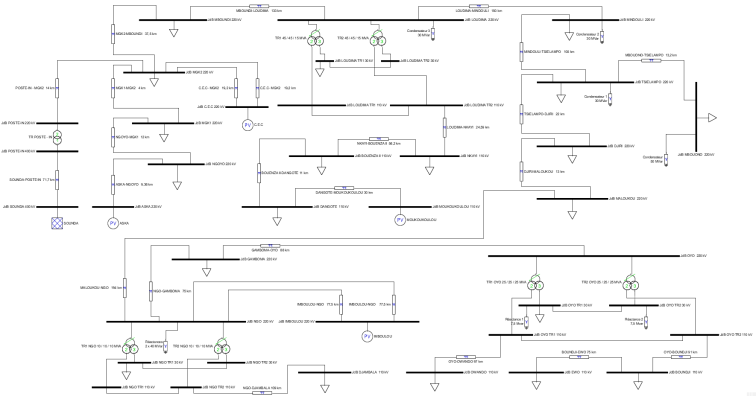
Figure 1. Sounda Model Connected to the National Electricity Grid of Congo.
3. Mathematical Modelling of the Electricity GRID
3.1. Branch Impedance Parameters of the Network
A HV/EHV electric line is characterised by four distributed linear parameters: resistance R (Ω/km), inductance L (H/km), capacitance C (F/km) and leakage conductance G (S/km) .
Linear Parameters and Calculation Bases
The linear parameters of the lines presented in Table 3 are derived from E²C-Congo data :
Table 3. Linear Parameters of the lines.

400 kV lines (ACSR 455 mm²)

220 kV lines (ACSR 500 mm²)

110 kV lines (ACSR 500 mm²)

R1

0.030 Ω/km

0.050 Ω/km

0.058 Ω/km

L1

0.90 mH/km

1.00 mH/km

0.1133 mH/km

X1 = ω·L1

0.2827 Ω/km

0.3142 Ω/km

0.356 Ω/km

C1

12 nF/km

11 nF/km

9.5× 10-7S/km

B1= ω·C1

3.770×10⁻⁶ S/km

3.456×10⁻⁶ S/km

3.0× 10-6S/km

Impedances are converted to per-unit values on the base Sbase = 100 MVA :
Zpu= ZΩZbaseZbase(400kV) =4002100= 1600 Ω
Zbase (220kV) = 484 ΩZbase(110kV) = 121 Ω
Bpu= Bs/phase × Zbase = ω.C1.l. Un2/Sbase
The impedance parameters for all branches of the Congolese grid are listed in Table 4:
Table 4. Impedance Parameters of All Branches of the Congolese Electricity Grid.

Branch

Voltage (kV)

Length (km)

R (p.u)

X (p.u)

B (p.u)

SOUNDA–POSTE-IN

400

71.7

0.00134

0.01267

0.4325

POSTE-IN-MGK2

220

14.0

0.00145

0.00909

0.0234

AKSA-NGOYO

220

9.36

0.00097

0.00608

0.0157

NGOYO-MGK1

220

12.0

0.00124

0.00779

0.0201

MGK1-MGK2

220

4.0

0.00041

0.00260

0.0067

C.E.C-MGK2 (×2)

220

19.2

0.00198

0.01246

0.0321

MGK2-MBOUNDI

220

37.5

0.00387

0.02434

0.0627

MBOUNDI-LOUDIMA

220

133.0

0.01374

0.08633

0.2225

LOUDIMA-MINDOULI

220

150.0

0.01550

0.09736

0.2509

MINDOULI-TSIELAMPO

220

105.0

0.01085

0.06815

0.1756

TSIELAMPO-DJIRI

220

22.0

0.00227

0.01428

0.0368

DJIRI-MALOUKOU

220

13.0

0.00134

0.00844

0.0217

MALOUKOU-NGO

220

194.0

0.02004

0.12592

0.3245

NGO-GAMBOMA

220

75.2

0.00777

0.04881

0.1258

GAMBOMA-OYO

220

87.6

0.00905

0.05686

0.1465

IMBOULOU-NGO (×2)

220

77.5

0.00801

0.05030

0.1296

MBOUONO-TSIELAMPO

220

13.2

0.00136

0.00857

0.0221

OYO-OWANDO

110

97.0

0.04650

0.28539

0.0352

OYO-BOUNDJI

110

91.0

0.04362

0.26774

0.0330

BOUNDJI-EWO

110

75.0

0.03595

0.22066

0.0272

LOUDIMA-NKAYI

110

24.59

0.01179

0.07235

0.0089

NKAYI-BOUENZA II

110

56.2

0.02694

0.16535

0.0204

BOUENZA II-DANGOTE

110

11.0

0.00527

0.03236

0.0040

DANGOTE-MOUKOUKOULOU

110

30.0

0.01438

0.08826

0.0109

NGO-DJAMBALA

110

109.0

0.05225

0.32069

0.0396

3.2. Modelling of Network Elements
3.2.1. Generator Model
The generator is considered the starting point of the electricity grid. It ensures the production of electrical energy demanded by consumers. In power flow analysis, the generator is modelled as a constant voltage source Vg that injects generated active power Pg and reactive power Qg as illustrated in Figure 2 . The reactive power of the generator adjusts to maintain the voltage at node i within the admissible range, characterised by reactive power limits Qgmin and Qgmax.
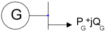
Figure 2. Generator model.
The Sounda plant alternator is modelled by an internal electromotive force E'  behind a transient reactance Xd'. The active and reactive powers injected at the PV generator node are :
PG =(E' V /Xd')sinδ(1)
QG =(E' V cosδ-V2)/Xd'(2)
where δ is the load angle (angle between E'  and V) and V the terminal voltage. Static stability requires |δ| < 90° .
3.2.2. Transmission Line Model
A section of an electric power transmission line between nodes i and k can be represented by the π-equivalent circuit as illustrated in Figure 3:
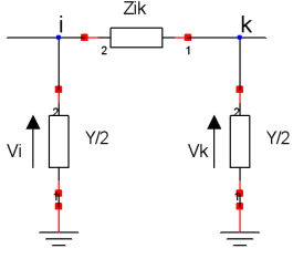
Figure 3. Transmission Line Model (π-equivalent circuit).
ZikLine impedance,
 Zik=  Rik+j  Xik(3)
Rik and  Xik are respectively the resistance and reactance of the line between buses i and Yi and Yk, and are the shunt admittances.
Y̅i =Y̅k = Gi-jBi (4)
3.2.3. Load Model
The electrical load is modelled as constant active power P ch and reactive power Q ch absorption . This load typically represents a transformation substation supplying distribution networks (Figure 4).
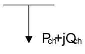
Figure 4. Electrical Load Model.
3.2.4. Shunt Element Model
Shunt elements (capacitor banks or reactors) are inserted in the network to supply reactive power Qc or absorb reactive power Qind, in order to achieve a better voltage profile (Figure 5).
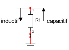
Figure 5. Shunt Element Model.
3.2.5. Two-winding Transformer Model
Parameters being referred to the secondary side, the transformer can be represented as in Figure 6 :
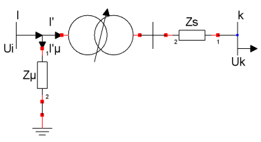
Figure 6. Two-Winding Transformer Model.
Zs=Uncc%.Un100.√3.In(5)
Zs=Rs + jXs(6)
Impedance referred to the secondary side.
Where
Rs= ZscosφT; Xs= ZssinφT et φT =tan-1(XR)(7)
Z̅µmagnetizing impedance of the transformer
3.2.6. Three-winding Transformer Model
The three-phase three-winding transformer is represented in Figure 7 , with impedances referred to the secondary (Z̅s2) and tertiary (Z̅s3) windings:
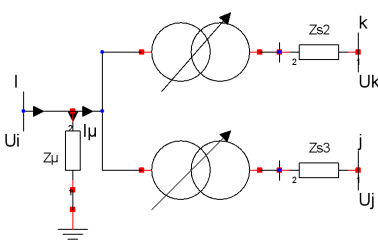
Figure 7. Three-Winding Transformer Model.
Z̅s2impedance referred to the secondary side
Z̅s3impedance referred to the tertiary side
Z̅µmagnetizing impedance of the transformer
With:Zs2=U12ncc%.Un100.√3.I1n(8)
Zs3=U13ncc%.Un100.√3.I1n(9)
The following expressions are then derived:
Rs2=Zs2cosφ12; Rs3=Zs3cosφ13(10)
Xs2=Zs2sinφs2; Xs3=Zs3sinφs3(11)
φs2=φs3=φ=tan-1(Xs2Rs2)(12)
3.3. General Equations of HV and EHV Lines
The study of long extra-high voltage lines requires consideration of the wave nature of energy transport. The line of length l must be represented as a circuit with distributed parameters, as shown in Figure 8 :
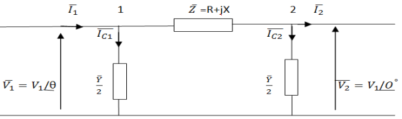
Figure 8. Equivalent Model of an EHV Line with Distributed Parameters.
The current at the sending end of the line is:
 ̅̅I = I1  - φ1φ1 (I1¯,V1¯)(13)
The current at the receiving end of the line is:
I2¯=I2  - φ2φ2 (I2¯,V2¯)(14)
The current flowing through the line is: I
Line impedance is:
Z¯ =R+jLω =R+jX Z  β [Ω](15)
Line admittance is:
Y¯ = jCω =Y 900 S(16)
Power Equations at Line Input and Load Terminals
The formulas corresponding to the apparent power (S1), the active power (P1) and the reactive power (Q1) at the source end of the line can be represented geometrically by the power triangle shown in Figure 9.
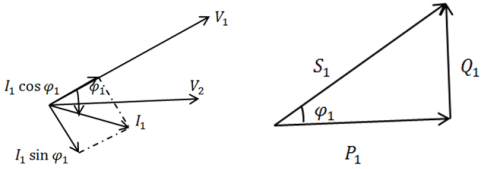
Figure 9. Voltage diagram and power triangle.
The three-phase active, reactive and apparent powers at the source (S₁) and at the load terminals (S₂) of a three-phase line are :
P1=3 U1.I1.cosφ1  W(17)
Q1=3 U1.I1.sinφ1  VAR(18)
S1¯=3 U1¯.I1*¯= P1+ jQ1  VA(19)
P2=3 U2.I2.cosφ2  W(20)
Q2=3 U2.I2.sinφ2  VAR(21)
S2¯=3 U2¯.I2*¯= P2+ jQ2  VA(22)
Active losses and reactive power consumed in the line :
P=3RI2; QL = 3 XL. I2 ; Qc = C.ω. U2 par phases (23)
 QLigne= 3 XI2 - (2 ). (U12+U22) (trois phases)(24)
3.4. Load Flow Calculation
3.4.1. Nodal Admittance Matrix Formulation
The nodal admittance matrix is composed of self-admittances yiiand transfer admittances  yik. The self-admittance «yii», associated with node «i», is equal to the sum of the admittances of all branches incident to that node. The transfer admittance «- yik», associated with nodes «i» and «k», is equal to the admittance of the branch connecting the two nodes, taken with a negative sign. Setting Yik= - yki, then, as in the case of self-admittances, the transfer admittances can be represented by the matrix [Yik]. For a system of n nodes :
I1I2In=Y11Y21Yn1 Y12Y22Yn2Y1nY2nYnn.V1V2Vn(25)
Equation (25) defines the matrix equation obeying Kirchhoff's current law (KCL) applied to an n-bus network .
With
[Y]=Y11Y21Yn1 Y12 Y22 Yn2Y1nY2nYnn(26)
is the n×n nodal admittance matrix of the network.
3.4.2. Network Node Equations
For a network with slack (Vφ), PV and PQ nodes, the complex power at node i is :
S̲i=V̲i.I̲i*(27)
At node i, KCL can be written as:
I̲i=Y̲ii.V̲i+i=1k1nY̲ikV̲i-V̲k(28)
S̲i=Y̲ii.V̲i2+V̲ii=1k1nY̲ik(V̲i-V̲k)(29)
Thus,
S̲i=P̲i+jQ̲i(30)
Where Pi and Qi are the active and reactive powers injected at node i. By expressing the real and imaginary components of the power injected at each node, we obtain :
P̲i=Y̲ii.V̲i2.cosαii+V̲i.i=1k1nY̲ik.V̲k.cos(φi-φk-αik)Q̲i=Y̲ii.V̲i2.sin-αii+V̲i.i=1k1nY̲ik.V̲k.sin(φi-φk-αik)(31)
After expansion:
P̲i=G̲ii.V̲i2+V̲i.i=1k1nV̲k. [G̲ik.cosφi-φk+B̲iisinφi-φk]Q̲i=-B̲ii.V̲i2+V̲i.i=1k1nV̲k. [G̲iksinφi-φk-B̲ikcosφi-φk](32)
Where φi, φk, αii and αik, are respectively the voltage angles at nodes «i» and « k », and the arguments of the self- and transfer admittances. By analogy, the voltage at each node «i» of the network can be expressed. Based on the power injected at node «i», we have:
S̲i*=V̲i*.I̲i=V̲i*. i=1k1nY̲ik.V̲k=Y̲ii.V̲i.V̲i*+V̲i*.i=1k1nY̲ik.V̲k(33)
V̲i=1Y̲ii [S̲i*V̲i*-i=1k1nY̲ik.V̲k](34)
For a network of «n» nodes, the voltage expression at each node can be written in the following matrix form:
[V̲i] = [Y̲ii] -1([S̲i*, V̲i*] -1-i=1k1nY̲ik.V̲k(35)
3.4.3. Power Flow Equations Between Two Nodes
Consider an element connecting nodes i and k as illustrated in Figure 10, the complex power flowing through this element can be written as a function of V̲i and V̲k at its two terminals. The power flowing from i to k is given by:
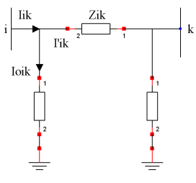
Figure 10. Line model.
I̲ik=I̲ik'+I̲oik(36)
With
I̲ik' = Y̲ikV̲i-V̲k, I̲oik=Y̲oik.V̲i(37)
I̲ik=Y̲ikV̲i-V̲k+Y̲oik.V̲i(38)
S̲ik=V̲i. [Y̲ikV̲i-V̲k+Y̲oik.V̲i] *=V̲i. [Y̲ik*+Y̲oik*V̲i*-Y̲ik*.V̲k*](39)
S̲ik=Y̲ik*+Y̲oik*V̲i*. V̲i-Y̲oik*.V̲k*.V̲i(40)
S̲ik=Y̲ik*+Y̲oik*V̲i2-Y̲oik*. V̲i.V̲k.ej(φi-φk)(41)
Thus:
Y̲ik=Gik+jBik Y̲oik=Gik+jBik Y̲ik*=Gik-jBikY̲oik*=Goik-jBoik(42)
S̲ik=Gik-jBik+Goik-jBoik.Vi2-Vk.Vi.ejφi-φk. [Gik-jBik](43)
Setting:
G'̲ik=Gik+jGoik B'̲oik=Bik+jBoik(44)
S̲ik=G'ik-jB'oikV̲i2-Vi.Vk.cosφi-φk+jsinφi-φk. [Gik-jBik](45)
S̲ik=G'ik-jB'oikV̲i2-Vi.Vk. [Gik.cosφi-φk+jGik.sinφi-φk-jBikcosφi-φk+Bik.sinφi-φk(46)
S̲ik=Pik+jQik,
The expressions for the active and reactive power are obtained:
Pik=G'ik.Vi2-Vi.Vk.Gik.cosφi-φk+Bik.sinφi-φkQik=-Bik.Vi2-Vi.Vk. [Gik.sinφi-φk-Bik.cosφi-φk](47)
When power flows from node k to node i, we obtain:
Pki=G'ki.Vk2-Vi.Vk.Gki.cosφk-φi+Bki.sinφk-φiQki=-B'ki.Vk2-Vi.Vk. [Gki.sinφk-φi-Bki.cosφk-φi](48)
3.4.4. Power Loss Equations
From equations (47) and (48), the losses through a branch element are :
Pi=Pik+Pki=G'ki.(Vi2+Vk2)-2Gki.Vi.Vkcosφi-φkQi=Qik+Qki=-B'ki.(Vi2+Vk2)+2Vi.Vk.Bki.cosφi-φk] (49)
3.4.5. Power Flow Methods
The power grid equations obtained are nonlinear in nature; their resolution therefore requires efficient methods to obtain reliable results. The methods recognised for solving such equations are highly varied, with differing levels of effectiveness. Indeed, several methods exist, namely the direct current (DC) method, the continuation method, the Gauss-Seidel method, and global methods such as the Newton-Raphson method .
Newton-Raphson Method
For this method, we assume that the active powers Pi and reactive powers Qi are known quantities, while the unknowns are the voltage magnitude Vi and phase angle φi. The parameters are initialised by selecting, at the outset, approximate values for the voltages and phase angles at each bus :
V10,V20, …,Vn0 and φ10,φ20, …,φn0;
From these initial values, the active and reactive powers withdrawn at each bus can be calculated:
P10,P20, …,Pk0,…Pn0 and Q10,Q20, …,Qk0,…Qn0;
Using the nodal equations (34), the power mismatches at each bus are computed:
Pi0=Pid-Pi0; Qi0 =Qid-Qi0(50)
These expressions can be written in the following matrix form:
Pi0Qi0=PidQid-Pi0Qi0(51)
where Pid and Qid are the specified active and reactive powers at bus i; they are fixed quantities. The norm of the error vectors Pi and Qi is computed as:
Pi=MaxPi et Qi=MaxQi(52)
Let:
Pid=Pi0+∆Pi1(53)
Where:
∆Pi1=k=1n∂Pi∂Vk∆Vk+k=1n∂Pi∂φk∆φk(54)
Pi0=PiV10, V20,…,Vk0,…,Vn0φ10,φ20,…,φk0,…,φn0(55)
Similarly, for reactive power:
Qid=Qi0+∆Qi1(56)
Where:
∆Qi1=k=1n∂Qi∂Vk∆Vk+k=1n∂Qi∂φk∆φk(57)
Qi0=QiV10, V20,…,Vk0,…,Vn0φ10,φ20,…,φk0,…,φn0(58)
Equations (54) and (57) in matrix form can be written as follows:
∆P1∆P2∆Pi∆Q1∆Q2∆Qi=∂P1∂V1∂P2∂V1∂Pi∂V1∂Q1∂V1∂Q2∂V1∂Qi∂V1 ∂P1∂V2∂P2∂V2∂Pi∂V2 ∂Q1∂V2∂Q2∂V2∂Qi∂V2   ∂P1∂Vi∂P2∂Vi∂Pi∂Vi ∂Q1∂Vi∂Q2∂Vi∂Qi∂Vi 1V∂P1∂φ11V∂P2∂φ11V∂Pi∂φ1 1V∂Q1∂φ11V∂Q2∂φ11V∂Qi∂φ1 1V∂P1∂φ21V∂P2∂φ21V∂Pi∂φ1 1V∂Q1∂φ21V∂Q2∂φ21V∂Qi∂φ1   1V∂P1∂φi1V∂P2∂φi1V∂Pi∂φi 1V∂Q1∂φi1V∂Q2∂φi1V∂Qi∂φi∆V1∆V2∆Vi∆φ1∆φ2∆φi(59)
3.4.6. Busbar Classification
The load flow problem of a power network is correctly formulated when a specific type of constraint is defined at each network bus .
The different bus types defined according to the network constraint types are presented in Table 5.
Table 5. Busbar Type Constraints of Congolese National Grid.

Busbar Type

Known Variables

Unknown Variables

Nodes

Load (P, Q)

P, Q

V, φ

20 HTB substations (Ngoyo, MGK1/2, Mboundi.)

Control (P, V)

P, V

Q, φ

C.E.C, AKSA, Imboulou, Moukoukoulou

Reference (slack)

V, φ

P, Q

Sounda 400 kV Bus

4. Simulation Results and Discussions
The national network, simulated under PSAT 2.1.11 (Power Systems Analysis Toolbox ) is a model comprising 45 buses in total, including one slack bus at Sounda (V₁ = 1.0 p.u., φ₁ = 0°); four PV buses: C.E.C, AKSA, Imboulou, Moukoukoulou; twenty EHV load buses (PQ); and twenty internal buses corresponding to the secondary and tertiary windings of the three-winding transformers at NGO, OYO and Loudima, as well as the parallel bus bars at the main substations. These internal buses have no load or source assigned in PSAT; they serve solely to model the three-winding transformer topology.
4.1. Network Voltage Behavior
The evolution of nodal voltages during the interconnection of Sounda to the Congolese power grid under the different scenarios is illustrated in Figures 11, 12 and 13. A numerical illustration of the voltages is also presented in Table 6 (see Appendix).
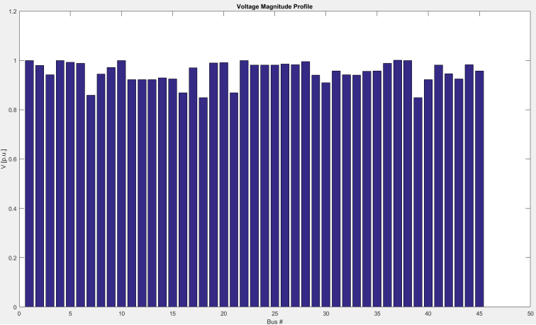
Figure 11. Network voltage profile curve (Scenario 1: full grid with C.E.C and AKSA).
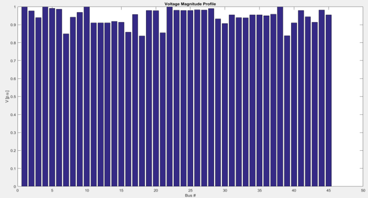
Figure 12. Voltage Profile Curve without Thermal Plants (Scénario 2).
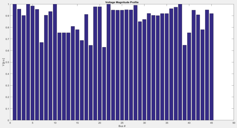
Figure 13. Voltage Profile Curve (Scenario 3: C.E.C at one-third power).
Interpretation
The voltage profile curve in Figure 11 of the complete network scenario shows two distinct zones. The Pointe-Noire area (AKSA, C.E.C, NGOYO, MGK1, MGK2: voltage ranging from approximately 0.990 to 1.000 p.u.) benefits from voltage support provided by C.E.C and AKSA, which helps maintain voltages close to the nominal level . The Poste-IN and MBOUNDI zone exhibits satisfactory voltages (0.970–1.001 p.u.). In contrast, the central network zone (Loudima, Mindouli, Tsielampo, Maloukou, Mbouono, Djiri) shows voltages between 0.822 and 0.922 p.u., all below the regulatory limit of 0.95 p.u. . This is due to the absence of local reactive compensation in this area and the long transmission lines (Mboundi-Loudima 133 km, Loudima-Mindouli 150 km, Mindouli–Tsielampo 105 km). Along the northern axis (GAMBOMA, NGO, OYO, OWANDO, BOUNDJI, EWO), voltages vary between 0.909 and 0.981 p.u. Eleven buses are under voltage.
Figure 12 shows an even more degraded overall voltage profile. In the absence of thermal plants, voltage profiles exhibit greater nodal dispersion. Some buses far from Sounda record voltages below 0.95 p.u., indicating a risk of voltage collapse if no reactive compensation is added . The central zone voltages (Mindouli 0.838 p.u., Tsielampo 0.821 p.u., Maloukou 0.843 p.u., Mbouono 0.820 p.u., Djiri 0.833 p.u.) are particularly low, signaling collapse risk . The use of Continuation Power Flow (49 iterations, versus 6 for Sc1) indicates that the classical Newton–Raphson method diverges for this scenario. Sounda generates 453.1 MW (4.531 p.u.), Imboulou 91.6 MW, and Moukoukoulou 56.5 MW. The total generation of 601.2 MW exceeds the load of 530.7 MW, but losses reach 70.5 MW (11.7%), a very high rate revealing poor voltage profiles across the network. Twelve buses are under voltage.
Figure 13 reveals the most degraded profile of the study. Unlike Scenario 2, where Newton-Raphson diverged, Newton–Raphson converges in 7 iterations in Scenario 3, meaning equilibrium exists but at extremely low voltages. Voltages remain around 0.97–1.00 p.u. because AKSA (124.7 MVAR), Moukoukoulou (74 MVAR), and C.E.C (150 MW + 345 MVAR) provide strong reactive support in this zone. However, CEC’s active generation is reduced to one-third of Scenario 1, forcing Sounda to transmit an additional 228 MW on the Sounda-POSTE-IN line, increasing losses. The voltage profile shows a critical central zone, with voltages collapsing to alarming levels: Mindouli (0.629 p.u.), Mbouono (0.646 p.u.), Tsielampo (0.647 p.u.), Djiri (0.670 p.u.), Maloukou (0.688 p.u.). These values are below the 0.95 p.u. threshold, more critical than Scenario 2, as Sounda supplies this central zone via long 388 km radial lines with high losses depressing voltages. Along the northern axis (buses 19–27, OYO–OWANDO-BOUNDJI-EWO), voltages range from 0.868 to 0.936 p.u., all below 0.95 p.u. Gamboma (0.936 p.u.) and Mboundi (0.911 p.u.) are newly under voltage compared to Scenario 1. Scenario 3 presents more under-voltage buses than the all-hydraulic configuration, despite partial support from C.E.C.
4.2. Active Power Behavior
The active power distribution in the network for the three scenarios is presented in Figures 14, 15 and 16.
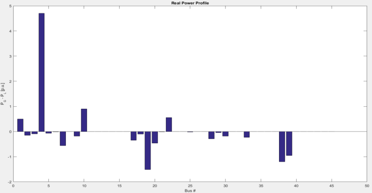
Figure 14. Active Power Flow Curve (Scenario 1).
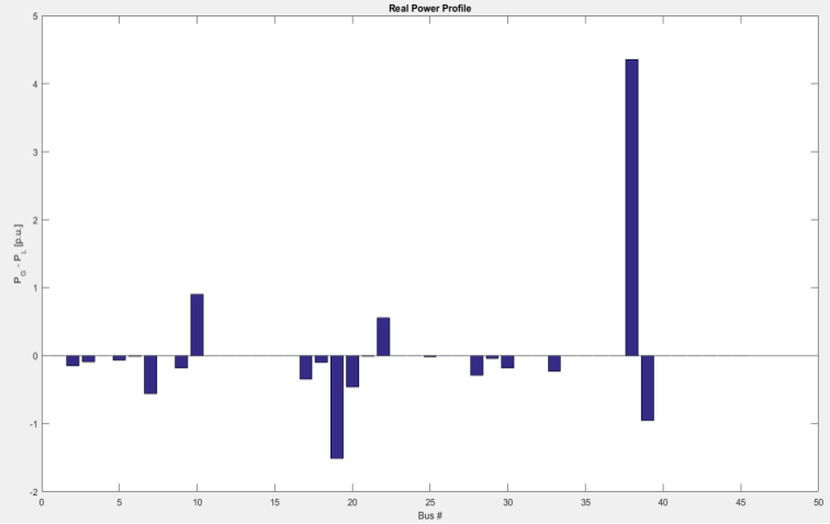
Figure 15. Active Power Flow Curve (Scenario 2).
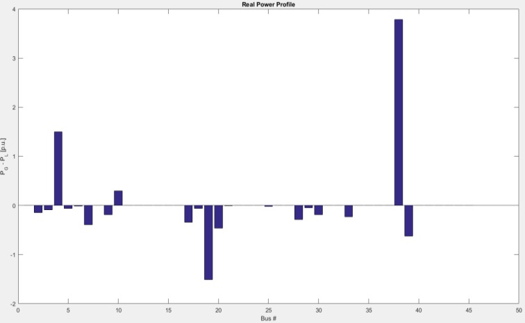
Figure 16. Active Power Flow Curve (Scenario 1).
Interpretation
Figure 14 represents the distribution of active power flows across network branches. The active power distribution curve shows that C.E.C (470 MW) assumes the majority of generation. Flows on the main lines from POSTE-IN to MGK2 reach 4.1478 p.u. = 414.78 MW (line 25, PSAT). The power flow on the SOUNDA-POSTE-IN line is only −1.1988 p.u. in absolute value because Sounda, as the slack bus, absorbs the surplus of 119.9 MW from other generators (C.E.C + AKSA + Imboulou + Moukoukoulou = 665.5 MW > load + losses = 545.6 MW). In PSAT simulation, Sounda is the slack bus whose power is calculated by balance. A negative value means the sum of other generators (CEC 470 + AKSA 50 + Imboulou 90 + Moukoukoulou 55.5 = 665.5 MW) exceeds demand (521.6 MW) + losses (24.0 MW) = 545.6 MW . The surplus of 119.9 MW is assigned to the slack bus as negative power. In real operation, this means C.E.C or AKSA output must be reduced to balance the system, as in Scenario 3.
In the all-hydraulic configuration, Continuation Power Flow (49 iterations, versus 6 for Scenario 1) indicates classical Newton–Raphson divergence. According to Figure 15, Sounda generates 453.1 MW (4.531 p.u.), Imboulou 91.6 MW, and Moukoukoulou 56.5 MW. The total generation of 601.2 MW exceeds the load of 530.7 MW, but losses reach 70.5 MW (11.7%), a very high rate revealing poor voltage profiles across the network. Without thermal input, Sounda supports the entire active load of the network. Power flows increase on all lines, with potential saturation of certain branches. Active losses rise compared to the thermal scenario, due to longer flows between Sounda and load centers. This result highlights the need to reinforce the transmission network for Sounda’s commissioning.
Only three active generators appear in Figure 16. Bus 38 (SOUNDA, ~3.78 p.u. = 378 MW) dominates production with 67.7% of total generation. Bus 4 (C.E.C) contributes 26.9%. Bus 10 (IMBOULOU) contributes 5.4%. AKSA (bus 1) and Moukoukoulou (bus 22) have zero active generation. This strong concentration of generation at Sounda (67.7%) explains the high losses, as Sounda must transmit 378 MW over very long lines .
4.3. Reactive Power Behavior
The reactive power flow in the network for the three scenarios is described in Figures 17, 18 and 19.
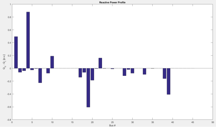
Figure 17. Reactive Power Flow Curve of the Network (Scenario 1).
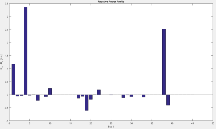
Figure 18. Reactive Power Flow Curve (Scenario 2).
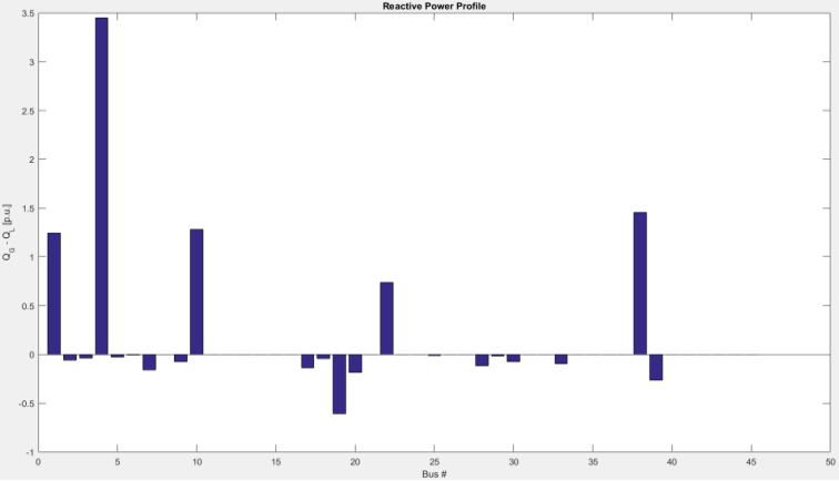
Figure 19. Reactive Power Flow Curve (Scenario 3).
Interpretation
Figure 17 shows reactive power behavior in the interconnected network. The Sounda alternator, operating in reactive generation mode, compensates for reactive needs of HV lines and loads. Positive reactive exchanges are observed at line beginnings and negative at line ends, characteristic of the Ferranti effect. Excitation adjustment of generator units maintains a power factor close to unity .
Figure 18 reveals significantly higher reactive power requirements in this scenario. Long lines consume more reactive power, and terminal buses show major reactive deficits. This highlights the need to install capacitor banks or static VAR compensators (SVC) at strategic points in the network to ensure voltage stability in the absence of thermal plants.
Figure 19 reveals the unprecedented reactive balance of Scenario 3. Five reactive generation buses appear, all injecting positively (over-excitation). Bus 4 (C.E.C) dominates with Q ≈ 3.45 p.u. = 345 MVAR, meaning C.E.C, though producing only 150 MW active, massively injects 345 MVAR reactive to support voltage in the Pointe-Noire zone. This is consistent, as a CCGT turbine can inject 70–80% of its nominal power in reactive even at low active load . Bus 1 (AKSA, Q ≈ 1.25 p.u. = 125 MVAR) and bus 22 (Moukoukoulou, Q ≈ 0.74 p.u. = 74 MVAR) confirm their role as synchronous condensers. Despite these massive injections (total reactive = 817.1 MVAR), the central zone remains under voltage because reactive power generated at Pointe-Noire (AKSA + C.E.C ≈ 470 MVAR) cannot traverse the 388 km radial line without reactive losses .
5. Discussions
The most concerning result from PSAT simulations is the identification of at least 11 busbars under voltage in all three scenarios, including with C.E.C and AKSA in service . The most critical nodes are Mbouono (V = 0.848 p.u.), Tsielampo (V = 0.849 p.u.) and Djiri (V = 0.859 p.u.) . These under-voltages result from the radial (linear) structure of the network along the Mboundi-Loudima-Mindouli-Tsielampo axis over 388 km without intermediate local generation, and from the high inductive reactive load of HTB substation transformers . The existing capacitors (3 ×30 MVAR) are woefully insufficient. Additional reactive compensation in the central zone (Mindouli, Tsielampo, Maloukou substations) is imperative to bring voltages above 0.95 p.u. .
Furthermore, the recourse to the continuation power flow (49 iterations, PSAT) for Scenario 2 demonstrates that the grid cannot operate stably without C.E.C and AKSA with the current load configuration. The divergence of classical Newton-Raphson is a formal indicator of crossing the saddle-node bifurcation (SNB) boundary . This means no stable grid equilibrium exists without thermal plants under current parameters. C.E.C and the Djeno/AKSA gas turbine are therefore not optional sources but necessary conditions for system stability .
Moreover, the current national grid load demand with losses is approximately 545.6 MW, and the energy production of Congo before Sounda's integration already exceeds this demand. Sounda cannot operate at its full nominal capacity of 800 MW in any of the three proposed scenarios (−1.1988 p.u. for Scenario 1, 4.531 p.u. for Scenario 2, and 3.78 p.u. for Scenario 3), except with a regional interconnection through the ECCAS Energy Pool (PEAC) .
6. Conclusions
This article has presented the modelling of the national power grid of Congo-Brazzaville incorporating the Sounda Gorges power plant. Three network scenarios comprising 45 buses, 27 lines and 19 transformers were simulated under PSAT 2.1.11 and analysed through 9 profile Figures. The PSAT results reveal:
1) In the full configuration (Scenario 1), the identification of 11 buses out of 45 exhibiting undervoltage (< 0.95 p.u.) , including MBOUONO (0.848), TSIELAMPO (0.849) and MINDOULI (0.869), despite the presence of CEC and AKSA.
2) The indispensability of C.E.C and AKSA to the viability and stability of the network: the all-hydro configuration required a continuation power flow (49 iterations), indicating operation beyond the stability limit .
3) It also emerges from this study that Sounda will not be able to operate at its full rated capacity of 800 MW, since the current load demand of the Congolese national grid, including losses, is approximately 545.6 MW, which is already lower than the output of the existing power plants prior to Sounda's integration. Consequently, a portion of the output from the Sounda power plant will need to be exported through an interconnection to the Central African Power Pool (CAPP/PEAC) .
The priority recommendations are: reactive power compensation at the Mindouli, Tsielampo and Maloukou substations (STATCOM or capacitor banks) ; mandatory continued operation of C.E.C and AKSA to guarantee static stability ; and the export of Sounda's output to the CAPP/PEAC.
Abbreviations

PSAT

Power Systems Analysis Toolbox

EEC

Congolese Electric Energy

SNE

National Electricity Company

C.E.C

Congo Electric Plant

GT

Gas Turbine

CCGT

Combined-cycle Gas Turbine

HV

High Voltage

EHV

Extra High Voltage (Very High Voltage)

PEAC

Central Africa Energy Pool (CAPP)

PQ

Load Bus -active Power P and Reactive Power Q Specified

PV

Generator Bus-active Power P and Voltage Magnitude V Specified

p.u

Per-unit (Normalised Value, Base 100 MVA / Rated Voltage)

MVA

Megavolt-Ampere (Apparent Power)

MW

Megawatt (Active Power)

MVAR

Megavar (Reactive Power)

Acknowledgments
The authors thank the GEA Laboratory (ENSP-UMNG), E²C company and ISTA-Kinshasa for technical data and access to the PSAT 2.1.11 simulator.
Author Contributions
Yves Pancrace Bowassa-Bob: Conceptualization, Data curation, Formal Analysis, Funding acquisition, Investigation, Methodology, Project administration, Visualization, Writing – original draft
Rodolphe Gomba: Data curation, Investigation
Flory Lidinga Mobonda: Formal analysis, Project administration, Supervision
Christian Vunda Ngulumingi: Methodology, Software, Resources
Timothee Nsongo: Funding acquisition, Methodology, Validation, Writing – review & editing
Andre Pasi Bengi Masata: Methodology, Validation, Writing – review & editing
Verlan Chrice Ikama: Software, Visualization
Conflicts of Interest
The authors declare no conflicts of interests.
Appendix
Table 6. Nodal Voltage Profile -Comparative Table: PSAT (V in p.u.), Critical Busbars <0.95 p.u.

Busbars

Scenario 1 (V)

Scenario 2 (V)

Scenario 3 (V)

Threshold

Type

SOUNDA 400 kV (slack)

1.000

1.000

1.000

≥0.95

Slack

CEC 220 kV

1.000

1.000

1.000

PV

PV

AKSA 220 kV (TAG Djeno)

1.000

1.000

1.000

PV

PV

IMBOULOU 220 kV

1.000

1.000

1.000

PV

PV

MOUKOUKOULOU 110 kV

1.000

1.000

1.000

PV

PV

POSTE-IN 220 kV

1.001

0.949

1.000

0.95

PQ

NGOYO 220 kV

0.995

0.989

1.000

0.95

PQ

MGK2 220 kV

0.991

0.974

0.990

0.95

PQ

MGK1 220 kV

0.990

0.976

0.976

0.95

PQ

MBOUNDI 220 kV

0.970

0.951

0.911

0.95

PQ

BOUENZA II 110 kV

0.979

0.976

0.976

0.95

PQ

DANGOTE 110 kV

0.992

0.991

0.991

0.95

PQ

NKAYI 110 kV

0.940

0.925

0.911

0.95

PQ

LOUDIMA 220 kV

0.922

0.897

0.753

0.95

PQ

MINDOULI 220 kV

0.869

0.838

0.629

0.95

PQ

TSIELAMPO 220 kV

0.849

0.821

0.647

0.95

PQ

MALOUKOU 220 kV (Braz.)

0.869

0.843

0.688

0.95

PQ

MBOUONO 220 kV

0.848

0.820

0.646

0.95

PQ

DJIRI 220 kV

0.859

0.833

0.670

0.95

PQ

DJAMBALA 110 kV

0.989

0.984

0.984

0.95

PQ

GAMBOMA 220 kV

0.971

0.965

0.936

0.95

PQ

NGO TR2 (load)

0.981

0.976

0.976

0.95

PQ

OYO TR2 (load)

0.940

0.933

0.920

0.95

PQ

OWANDO 110 kV

0.909

0.901

0.868

0.95

PQ

BOUNDJI 110 kV

0.942

0.934

0.902

0.95

PQ

EWO 110 kV

0.945

0.937

0.905

0.95

PQ

References
[1] P. Kundur, Power System Stability and Control. New York: McGraw-Hill (EPRI), 1994.
[2] Bowassa-Bob, Y. P., Lidinga Mobonda, F., Ngoma Mvoundou, C., Pasi Bengi Masata, A. and Nsongo, T. (2026) Modeling of Hydrodynamic Parameters of the Kouilou-Niari River for Energy Efficiency of the Sounda Gorges Hydroelectric Power Plant in Republic of Congo. Journal of Power and Energy Engineering, 14, 59-81.
[3] E²C (Congolese Electric Energy), Annual Report on Electricity Production and Distribution. Brazzaville: E2C, 2021.
[4] W. F. Tinney and C. E. Hart, “Power Flow Solution by Newton’s Method,” IEEE Transactions on Power Apparatus and Systems, vol. PAS-86, no. 11, pp. 1449–1460, Nov. 1967.
[5] V. Ajjarapu and C. Christy, The continuation power flow: a tool for steady state voltage stability analysis, in IEEE Transactions on Power Systems, vol. 7, no. 1, pp. 416-423, Feb. 1992.
[6] F. Milano, “An Open Source Power System Analysis Toolbox,” IEEE Transactions on Power Systems, vol. 20, no. 3, pp. 1199–1206, Aug. 2005.
[7] IEC 60193: 2019, Hydraulic Turbines, Storage Pumps and Pump-Turbines-Model Acceptance Tests, 3rd ed. International Electrotechnical Commission, Geneva, 2019.
[8] C. C. Warnick, Hydropower Engineering. Prentice-Hall, Englewood Cliffs NJ, 1984.
[9] B. M. Weedy, B. J. Cory, N. Jenkins, J. Ekanayake and G. Strbac, Electric Power Systems. Wiley, 5th ed., 2012.
[10] J. D. Glover, M. S. Sarma and T. J. Overbye, Power Systems Analysis and Design, 6th ed. Cengage Learning, 2017.
[11] N. G. Hingorani and L. Gyugyi, Understanding FACTS: Concepts and Technology of Flexible AC Transmission Systems. IEEE Press, New York, 2000.
[12] W. D. Stevenson, Elements of Power System Analysis, 4th ed. McGraw-Hill, 1982.
[13] H. Saadat, Power System Analysis. McGraw-Hill, 3rd ed., 2010.
[14] T. Van Cutsem and C. Vournas, Voltage Stability of Electric Power Systems. Kluwer Academic Publishers (Springer), Boston, 1998.
[15] EN 50160: 2010+A3: 2019, Voltage Characteristics of Electricity Supplied by Public Electricity Networks. CENELEC, Brussels, 2019.
[16] A. J. Wood, B. F. Wollenberg and G. B. Sheblié, Power Generation, Operation, and Control. Wiley, 3rd ed., 2014.
[17] Central Africa Power Pool, Project situation in the portfolio of the Central Africa Power Pool (CAPP) Luanda, 2024.
Cite This Article
  • APA Style

    Bowassa-Bob, Y. P., Gomba, R., Mobonda, F. L., Ngulumingi, C. V., Nsongo, T., et al. (2026). Impact of the Sounda Gorge Hydropower Plant on Power Flow and Voltage Stability of the Congo-Brazzaville Electrical Network Under PSAT. Science Journal of Energy Engineering, 14(2), 47-64. https://doi.org/10.11648/j.sjee.20261402.13

    Copy | Download

    ACS Style

    Bowassa-Bob, Y. P.; Gomba, R.; Mobonda, F. L.; Ngulumingi, C. V.; Nsongo, T., et al. Impact of the Sounda Gorge Hydropower Plant on Power Flow and Voltage Stability of the Congo-Brazzaville Electrical Network Under PSAT. Sci. J. Energy Eng. 2026, 14(2), 47-64. doi: 10.11648/j.sjee.20261402.13

    Copy | Download

    AMA Style

    Bowassa-Bob YP, Gomba R, Mobonda FL, Ngulumingi CV, Nsongo T, et al. Impact of the Sounda Gorge Hydropower Plant on Power Flow and Voltage Stability of the Congo-Brazzaville Electrical Network Under PSAT. Sci J Energy Eng. 2026;14(2):47-64. doi: 10.11648/j.sjee.20261402.13

    Copy | Download

  • @article{10.11648/j.sjee.20261402.13,
      author = {Yves Pancrace Bowassa-Bob and Rodolphe Gomba and Flory Lidinga Mobonda and Christian Vunda Ngulumingi and Timothee Nsongo and Andre Pasi Bengi Masata and Verlan Chrice Ikama},
      title = {Impact of the Sounda Gorge Hydropower Plant on Power Flow and Voltage Stability of the Congo-Brazzaville Electrical Network Under PSAT},
      journal = {Science Journal of Energy Engineering},
      volume = {14},
      number = {2},
      pages = {47-64},
      doi = {10.11648/j.sjee.20261402.13},
      url = {https://doi.org/10.11648/j.sjee.20261402.13},
      eprint = {https://article.sciencepublishinggroup.com/pdf/10.11648.j.sjee.20261402.13},
      abstract = {This article presents the mathematical modelling of the national power grid of the Republic of Congo-Brazzaville and its future behaviour following the integration of the Sounda Gorges hydroelectric power plant. The network is simulated using the PSAT 2.1.11 software on a model comprising 45 buses, 27 lines, 19 transformers and 5 generators. The nodal admittance matrix [Ybus] equations and the active power transit equations Pik and reactive power transit equations Qik are developed. Three scenarios are simulated: a full network configuration with the C.E.C and AKSA thermal power plants, a full network configuration with the Congo Electric Power Plant (C.E.C) operating at one-third of its rated capacity, and an all-hydro network configuration without the thermal power plants. The PSAT simulations reveal critical results for network planning, notably the presence of at least 11 out of 45 buses exhibiting voltages below the regulatory threshold of 0.95 p.u. across all three scenarios, regardless of the presence or absence of the C.E.C and AKSA thermal power plants. Sounda will only be able to operate at its full rated capacity of 800 MW with an interconnection to the Central African Power Pool (CAPP), given that the current national demand, including losses (545.6 MW), is lower than the total available generating capacity.},
     year = {2026}
    }
    

    Copy | Download

  • TY  - JOUR
    T1  - Impact of the Sounda Gorge Hydropower Plant on Power Flow and Voltage Stability of the Congo-Brazzaville Electrical Network Under PSAT
    AU  - Yves Pancrace Bowassa-Bob
    AU  - Rodolphe Gomba
    AU  - Flory Lidinga Mobonda
    AU  - Christian Vunda Ngulumingi
    AU  - Timothee Nsongo
    AU  - Andre Pasi Bengi Masata
    AU  - Verlan Chrice Ikama
    Y1  - 2026/06/18
    PY  - 2026
    N1  - https://doi.org/10.11648/j.sjee.20261402.13
    DO  - 10.11648/j.sjee.20261402.13
    T2  - Science Journal of Energy Engineering
    JF  - Science Journal of Energy Engineering
    JO  - Science Journal of Energy Engineering
    SP  - 47
    EP  - 64
    PB  - Science Publishing Group
    SN  - 2376-8126
    UR  - https://doi.org/10.11648/j.sjee.20261402.13
    AB  - This article presents the mathematical modelling of the national power grid of the Republic of Congo-Brazzaville and its future behaviour following the integration of the Sounda Gorges hydroelectric power plant. The network is simulated using the PSAT 2.1.11 software on a model comprising 45 buses, 27 lines, 19 transformers and 5 generators. The nodal admittance matrix [Ybus] equations and the active power transit equations Pik and reactive power transit equations Qik are developed. Three scenarios are simulated: a full network configuration with the C.E.C and AKSA thermal power plants, a full network configuration with the Congo Electric Power Plant (C.E.C) operating at one-third of its rated capacity, and an all-hydro network configuration without the thermal power plants. The PSAT simulations reveal critical results for network planning, notably the presence of at least 11 out of 45 buses exhibiting voltages below the regulatory threshold of 0.95 p.u. across all three scenarios, regardless of the presence or absence of the C.E.C and AKSA thermal power plants. Sounda will only be able to operate at its full rated capacity of 800 MW with an interconnection to the Central African Power Pool (CAPP), given that the current national demand, including losses (545.6 MW), is lower than the total available generating capacity.
    VL  - 14
    IS  - 2
    ER  - 

    Copy | Download

Author Information
  • Polytechnic Superior National School (ENSP), Marien Ngouabi University, Brazzaville, Congo

  • Polytechnic Superior National School (ENSP), Marien Ngouabi University, Brazzaville, Congo

  • Laboratory of Electrical Engineering Department, Higher Institute of Applied Techniques-Kinshasa (ISTA-Kinshasa), Kinshasa, Democratic Republic of the Congo (DRC)

  • Laboratory of Electrical Engineering Department, Higher Institute of Applied Techniques-Kinshasa (ISTA-Kinshasa), Kinshasa, Democratic Republic of the Congo (DRC)

  • Faculty of Sciences and Techniques, Marien Ngouabi University, Brazzaville, Congo

  • Laboratory of Electrical Engineering Department, Higher Institute of Applied Techniques-Kinshasa (ISTA-Kinshasa), Kinshasa, Democratic Republic of the Congo (DRC)

  • Polytechnic Superior National School (ENSP), Marien Ngouabi University, Brazzaville, Congo