Abstract
We consider an iterative branching process in which an abstract object can subdivide into other objects. The multiplication process may be varied by the occurrence of random "fatal" events in which some of the subsequent objects or states may fail. The process is also constrained to terminate upon reaching a given number of events or alternatively upon reaching a fixed number of iteration steps. A system of diophantine integer-variable equations capable of describing the aforementioned process is proposed. These equations can be applied prospectively to many branching phenomena of physical, biological and demographic nature. The equations, which we call systems of equations S, Q, U can be reformulated into three main classes based on the behavior of the sum of variables with respect to a fixed principal numerical parameter (TC= 'Total Cases'). These systems always admit solutions and these are sought for the three classes. The mathematical properties of the three systems are presented both analytically and graphically, and the software script for calculating numerical solutions is attached. In the case of high TC values, where direct calculation is not possible, special solutions are also sought for the steady state case and the "most probable" case, the latter using statistical mechanics methods. Solutions examples are given for a wide range of TC parameters. We also refer to real-world examples of applications ranging from prey/predator population dynamics to population mortality modeling and 2d lattice space tiling and also tree leaves branching alternatives. The main purpose of the study here proposed is to implement a mathematical frame that can provide tools to be used in the study of real-world applications.
Keywords
Diophantine Equations, Binary Choices, Statistical Mechanics, Volterra-Lotka Equations, Demographic Mortality,
2d Lattice Partitions, Tree Leaves Branching
1. Introduction
Many branching processes of the most diverse types are present in the real physical world. Think, for example, of cell multiplication in biology, choice sequences, random motions, atomic nucleus fission, and even demographic issues like epidemic diffusion or population dynamics. Many of these cases are studied by resorting to probabilistic mathematical methods and/or techniques related to markovian processes or Monte-Carlo simulations or with models governed by feedback control laws (see e.g. the books in Ref
| [1] | M. Kimmel, D.E. Axelrod. "Branching processes in Biology", Springer, 2002. |
| [2] | S. Méléard, "Modèles aléatoires en Ecologie et Evolution", Springer, 2016. |
| [3] | N. Bacaer, "Histoires des mathematiques et de populations", ed. Cassini, Paris, 2008. |
[1-3]
). Also, more abstract objects like cellular automata or fractal processes (Ref.
| [4] | J. Kaandorp, "Fractal modelling growth and form in biology", Springer-Verlag, 1994. |
| [5] | A. Vulpiani, " Determinismo e caos", Carocci, 2004. |
[4, 5]
) can be involved and studied in branching iterations. In this study we will turn to a quite general mathematical formulation of a branching process based on integer variable equations (so-called diophantine equations) constrained to some boundary conditions. We will try to study the 'space' of all the exact equations solutions and their properties, without resorting to concatenated probabilistic assumptions. Our general branching process under study can be depicted as per
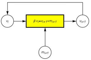
Figure 1:
Figure 1. A general branching process.
In the iterative process in
Figure 1, an initial number of identical v
i objects multiply themselves by a factor β (⩾2) generating β v
i objects. In the next iteration i+1 however a quota of the new β v
i objects can change in nature becoming objects no longer able to multiply. They amount numerically to a variable m
i+1 that can be considered as an input true random independent integer variable. This random nature of the m
i means that, considering the two parts integer partitions (including zero integer) of the β v
i, there are not 'preferred' partitions but all have the same random possibility to materialize. All these variables are defined by positive or null integers. Many real-life examples can be correlated to the process in
Figure 1: from the splitting and growth of biological organisms to the sequences of binary choices between alternatives etc. Coming back to the
Figure 1, two extreme cases can be contemplated: that in which the m
i are always null and then we will see an exponential growth v
i= β^i or the case in which we reach β v
i=m
i + 1 leading to v
i + 1=0, thus implying the end of the iterative process since there will be no more "fuel" for reproduction. Theoretically however, in addition to the stop possibility, the process in
Figure 1 could also proceed indefinitely or with unremitting growth or even coming to a stationary condition (as in the case of β=2 and m
i= v
i). This depends on the trend of the m
i variables. Moreover, we want to study what happens to the possible solutions (i.e. to the possible evolution paths of the process) when a termination condition is imposed on the overall process, that is, when an additional boundary condition is imposed. That is, we want to force into the process a termination condition that brings the process itself closer to the real cases (which cannot grow to infinity in size and time).
This condition will be:
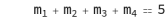
(1)
Where TC (i.e. "Total cases") is a parameter limiting the number of steps and the maximum total sum of objects m
i in the process evolution. In the following section we present the mathematical formulation of the problem and the definition of the different classes of equations (called S, Q, U classes) that arise in relation to how the eq. (
1) is met. In the following sections we will give a graphic visualization of the systems and then study the existence of particular solutions that might have important physical significance. Finally, some examples correlated to real cases are presented and some conclusions are drawn on the results achieved. For the numerical study, the value β = 2 will be used without loss of generality but with reduction of the weight of numerical calculations on the space of solutions. The results obtained with β = 2 will then be extendable to general values of β. The material here presented is based on studies performed by the author using personal resources and effort. As far as the author knows, this material is original. Many mathematical properties of the systems described are self-evident and are stated in Appendices as theorem statements. As a default approach, the proof of theorems is not provided in this context. This choice was made to avoid undue burden on the reader and to limit the size of the article.
2. The S, Q, U Equations
2.1. General Description
Recalling
Figure 1 and taking up some reasoning from Ref.
, we can then study the following recursive process in which we also assume β=2.
mi,vipositive or null integers(2)
Since we consider the m
i variables as independent, we can express v
i -by solving the first recursive eq. (
2)- as a function of the m
i sequence:
Now, the end-of-process condition of Eq. (
1) dictates that at step 'imax' there will be a termination of the process itself i.e. it will have to be v(imax)=0. This condition does not mean that the process cannot terminate even before 'imax', but it does mean that in any case at step 'imax' there will have to be a termination to the process. This means that:
That is, eliminating 2^imax and renaming 't' with 'i', we have:
(4)
and with equivalent form:
(5)
The S, Q, U systems of equations are based on the eq.s (
4) and (
5) with the addition of conditions derived by the eq. (
1):
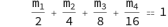
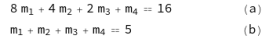
# The S system is defined with the addition of the condition:
;(6)
# The Q system is defined with the addition of the condition:
;(7)
# The U system is defined assuming no TC conditions on :
;(8)
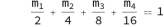
Examples:
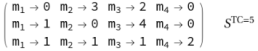
Assume e.g. TC=5, then we have:
# S system
# Q system

The search for all possible solutions of the above systems can help in understanding all possible branching behaviors. In the knowledge of the author-however- no explicit numerical solution formula is available for the equations systems presented. Therefore, numerical data and solutions have been detected with the aid of computer programs and applications. Of course, limitations are to be expected in the search due to the growing computational complexity when TC parameters grow. A computer software script designed by the author for the solutions search is given in Appendix I. The program runs under a mathematical computer application well known to scientific researchers. In finding solutions, it is also useful to check whether they have any rules or structures in their composition. This analysis was done in Appendix II for the three classes S, Q, U proposing some theorems useful in the analysis. Having knowledge of the entire range of solutions, one can ask whether there are one or more solutions that are representative of real situations and what conditions or methods should be introduced to find these preferred solutions. In the continuation of the study an attempt will be made to explore this issue further.
2.2. Some Systems Solutions
Solutions examples:
1) The simplest S system
Assume TC = 2 then imax =1 and the S system equation & solution will be:
2) The trivial solution
A trivial general solution is
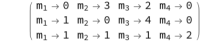
3) The TC = 5 solutions
In the S system case, the three solutions are:
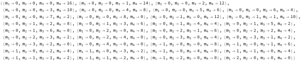
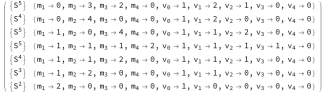
In the Q case, the solutions are seven:
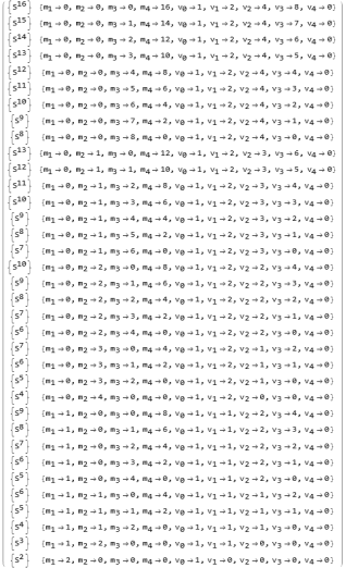
In the U case the 35 solutions are as follows:
4) The TC = 14 solutions
The S system equations in this case are (using the second equivalent form of the eq. (
5)):
and the solutions (total number 510) can be downloaded from the web site addressed at Ref.
| [7] | G. Alberti, Web site managed by the author and devoted to diophantine STC equation systems. https://squ-systems.eu |
[7]
.
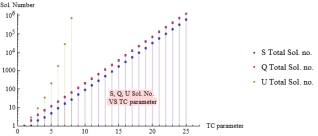
As can be seen from the examples above, the systems admit solutions, and these are limited in number, although increasing with TC. As a general rule, the solutions for the S system are included in the Q system solution space and, in turn, also the Q solutions are included in the U system solution set. This behavior and other properties of the highlighted systems are discussed in more detail in Appendix II. The U solutions set grows dramatically with TC (see data and plot below). A table and a plot of the number of distinct solutions for S, Q, U are given here. The solutions are computed with the script in Appendix I. Note that for the U column the data are limited to TC = 9 due to computational limits. As a general consideration we see that the three systems S, Q, U always admit a finite number of solutions. That number grows exponentially with the TC parameter in the case of S and Q while for U the growth is more than exponential (see
Figure 2 under the
Table 1).
Table 1. S, Q, U systems: no. of solutions vs TC.
TC | no. of solutions S | no. of solutions Q | no. of solutions U |
2 | 1 | 1 | 1 |
3 | 1 | 2 | 3 |
4 | 2 | 4 | 9 |
5 | 3 | 7 | 35 |
6 | 5 | 12 | 201 |
7 | 9 | 21 | 1827 |
8 | 16 | 37 | 27337 |
9 | 28 | 65 | 692003 |
10 | 50 | 115 | |
11 | 89 | 204 | |
12 | 159 | 363 | |
13 | 285 | 648 | |
14 | 510 | 1158 | |
15 | 914 | 2072 | |
16 | 1639 | 3711 | |
17 | 2938 | 6649 | |
18 | 5269 | 11918 | |
19 | 9451 | 21369 | |
20 | 16952 | 38321 | |
21 | 30410 | 68731 | |
22 | 54555 | 123286 | |
23 | 97871 | 221157 | |
24 | 175586 | 396743 | |
25 | 315016 | 711759 | |
26 | 565168 | 1276927 | |
Figure 2. S, Q, U different solutions number vs TC.
3. More on the Constrained Systems S, Q, U with β=2
To facilitate understanding of the structure of the systems of equations under discussion, it is useful to resort to a graphical representation of them as follows. This is done using the solutions highlighted in the previous paragraph. To graphically illustrate the associated branching process, we resort to the simple example of a single object initially, 'splitting' at later stages, generating other objects capable of multiplication. This situation can be represented by the cell multiplication thing in biology or-more generally-by the case of a single object making successive binary decisions. In the first case we will have the development of a population of objects in the second case we will have to consider all the possible subsequent choices and 'paths' taken by the object. In our branching process scheme, we also assume that during the growth process there may be individuals (or situations in the second object model) that are unable to split further; we will call these events 'fatal cases' in the process growth. They are the m
i objects introduced in the
Figure 1. We also introduce into our reasoning the parameter TC that imposes a termination with total constraint on the number of iterative steps allowed and also on the exact number of total deaths (system S). Or the TC parameter will be able to impose a limit constraint on the maximum number of steps and the maximum attainable number of deaths (system Q). Finally, there will be the case of system U in which only a constraint on maximum number of steps (imax= TC-1) will be imposed on the evolution of the system but with no constraints on the numbers of total 'fatalities'.
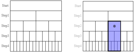
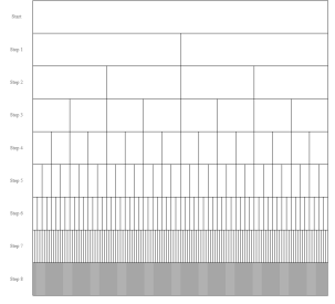
3.1. The STC=5 Case Graphical Description
Our analysis therefore put a constraint of process termination with conditions on the total number of elements involved. To clarify the pattern let us consider the simple case of TC = 5, with the possible solutions shown in the previous section. We have the following
Figure 3 where the possible iteration steps are four (TC-1=4).
Figure 3. Object splitting evolution with no-death events (left) and with a death event at step 2 (right).
In the figure we have chosen to represent the evolution of our branching case in the form of a binary choice case. Here we have a 'cell' element that -initially single- subdivides into two parts (left and right) in subsequent steps. This graphical artifice, which serves to compact the figure, is not a problem for our analysis, since we are not interested in the dimensional space growth but want to evaluate the 'cell' count that is preserved in our graph. The first part of
Figure 3 thus represents the development of a binary branching process without 'dead' elements within it. In the language of system S, we will say that we will have all m
i = 0. The process then expands indefinitely and at last step 4 we will have 16 elements. Instead, in the second part of
Figure 3 a 'deadly' event will occur, for example, on a cell in step 2. This cell (marked with a black dot) will no longer be able to reproduce - being "dead"- and then its potential progeny will also disappear. This effect on the progeny is represented by the shaded area under the deceased cell, which implies the elimination from the count of four of the 16 cells potentially predicted in step 4. Recall that the system S^(TC=5) is as follows:
and that its solutions are:
Now consider the following
Figure 4:
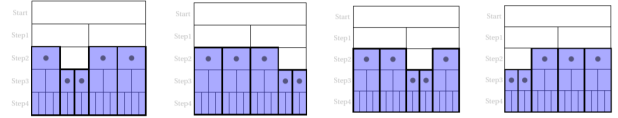
Figure 4. The four different instances of the same first solution for S^(TC=5).
We see that the first solution of the group S^(TC=5) is applicable for all the four possibilities shown in the figure. This means that each possible solution can correspond to several ways (which we can also call instances or configurations) of carrying out the process imposed by the solution. This is an important feature of S, Q, U binary systems and will be discussed below. The number of these possible configurations will also be computable (once the single specific solution is known) by combinatorial methods, as we shall see. To complete this graphic presentation, we also show in
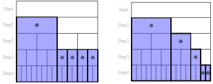
Figure 5 the other two solutions (choosing only one configuration of the several possible ones):
Figure 5. One instance for sol. II and sol. III for STC=5One instance for sol. II and sol. III for STC=5
Some other aspects are evident from these graphical representations. First, the nature of above equation (a) of the system is better understood. It dictates the fact that the process terminates at step 4 with all 16 final cells 'masked' by fatal events (direct or preceding). However, this equation (a) does not dictate the number of 'fatal' events; this number is constrained by equation (b). Indeed, we see that in all above graphs we have a complete 'masking' of the final cells (condition (a)) and the total number of 'dead' cells is always 5 (condition (b)). We also note another important feature: the total number of cells {vi}, i.e., the white cells below the initial start cell, is also always constant. This number is always equal to 3 in the case S^(TC=5), confirming, for β=2, the general rule (recalled in Appendix II) that is:
;(9)
3.2. The QTC=5 Case Build-up
As pointed out in the previous section and in more general terms in Appendix II, the case Q^(TC=5) contains all the solutions of S^(TC=2), (S^(TC=3)), (S^(TC=4)), (S^(TC=5)).
Figure 6 highlights these facts, where the first column shows the sub component (S^TC) for each solution. Also included in the table there are the {v
i} sequences related to the pattern of the {m
i} via eq. (
3). From these patterns it would then be possible to reconstruct figures and graphs similar to those shown in the previous section. Note also that in all cases the sequences terminate at step 4 when it is always v
4 = 0.
Figure 6. QTC=5 solutions, including STC<=5 solutions, with correlated vi cells.
3.3. The UTC=5 Case Build-up
Similarly, we show in
Figure 7 the 35 solutions of the system U^(TC=5) with highlighted in the first column the correspondence with an included sub-solution of type S. Again, the branching process ends at the fourth step. In this case, at most, the sub solutions come from systems S^16. This is in agreement with theorem T6 stated in Appendix II.
Figure 7. UTC=5 solutions, including S solutions, with correlated vi cells
3.4. The Cell/Decision Model and the Single Decision-making Model
We have already mentioned that our branching models can represent multiplying "populations" or a single "decider" object that chooses between two alternatives. In the case of the single decider, instead of seeing an abstract rectangular cell that is doubling, we will imagine a subject that has to decide between two alternatives, e.g. move left or right, stand still or go, generate the '0' bit or the '1' bit, etc. In this approach, each rectangle in the previous figures will be labeled accordingly ('left' or 'right,' etc.). In the course of decision sequences, the decision maker may encounter stopping situations or stopping "states" (our m-cases). The graphs in the previous subsections will then represent the space of possible paths with numerical constraints expressed by the solutions S, Q, U. This duality (cell/decision) of representation allows S, Q, U systems to be applied to many different cases and thus makes them flexible for applications.
4. Two 'Special' Solutions
With the aspects that emerged in the previous sections, we have seen that the constrained branching systems S, Q, U always admit solutions but the number of these solutions grows enormously as the value of the developed cases increases i.e. as the parameter TC increases. We have also seen that, wanting to compute all the solutions without having an explicit solving formula for the associated diophantine system, sooner or later we will run into computational capacity limit problems. If, however, we introduce into our reasoning some criteria for selection from among the totality of solutions, then it will be possible to simplify the mathematical calculation and thus identify some specific solutions that are more interesting or let us say 'special'. The two selection criteria we propose can be deduced from physics, namely, the criterion known in statistical mechanics of the 'most probable' solution on the one hand and the criterion of the stationary condition on the other. As before, we will start with the analysis of simpler cases and then extend the reasoning to more numerically complex cases. We will always consider the case β=2.
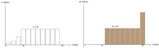
4.1. The "Steady State" Solution
In section 2 we reported the presence among the possible solutions of the systems S, Q, U of the trivial solution for the m variables: {1,1,1,....,1,2}. More generally it will be possible to have such structured solutions:
and for the {vi}:
In other words, the so-called "stationary" solution will start with v values growing exponentially until, at i=ia, a some-flat level is reached. From this point the {mi} and {vi} values will be the same and the 'solution' will have the shape of a rectangle function with bounds between 'ia' and 'ib'. In between, the variables will show the same constant value, except for the final step of the process where there will be a doubling of the constant value for {m
i} and a zeroing for {v
i} with termination of the sequence. The following
Figure 8 clarifies the general form of this solution.
Figure 8. The "steady state" solution shape with v and m variables almost constant for most part of the life cycle.
There will always be the possibility of obtaining S-systems with stationary solutions once the desired parameters and consequently the target TC are fixed, and vice versa. The following diophantine equation will govern the various possibilities and provide a calculation method for the solutions search.
(10)
With reference to
Figure 1 in the Introduction section, this solution clearly requires some form of control over the variables m
i+1, which can no longer be random. In fact, during the stationary phase, it must always be m
i+1=v
i for every (ia+1) ≤ i ≤ (ib-1). This condition is what is realized in real cases with automatic control mechanisms or in other real case with a self-equilibrium condition reaching. The final 'mortality' peak is here due only to the 'stop' condition that is imposed in our S, Q, U systems boundary conditions and sooner or later must be met.
4.2. The 'Most Probable' Solution Search Using Statistical Mechanics Methods
As before mentioned the (
4), (5), (6) eq.s not fully describe the binary choice S system possible evolutions sequences. If we indeed define
the (
4), (5), (6) equations will consider the total quantities of
mi, vi along the
i evolution steps, but these do not specify on which "cell" (or decision place), from the
Qi available, the effective 'deadly' events occur. See e.g. the "steady state" solution in the
Figure 5 (second graph). This is the solution that says that, for each step, a cell lives and the other dies, but it does not say where the dead event happen i.e. on the left or right cell of the two available at the
i level. Thus, for this only one simple solution we can have 2
3 = 8 possible sub-configurations or different paths sequences. The same condition holds for all the solutions of a S
TC system, in the sense that given a particular solution, one can wonder about the number of the associated configurations to this specific solution. This concept holds of course also for the Q
TC and the U
TC systems. Now, while we remember the exponential growth trend of the number of solutions in the above systems, this growth is again more enhanced for the possible associated configurations. Hereunder we try to directly compute the distribution of configurations associated with solutions from a case with limited TC.
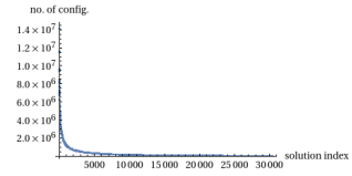
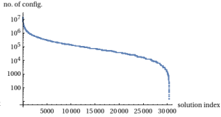
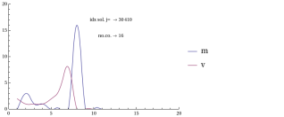
4.2.1. The TC=21 Case
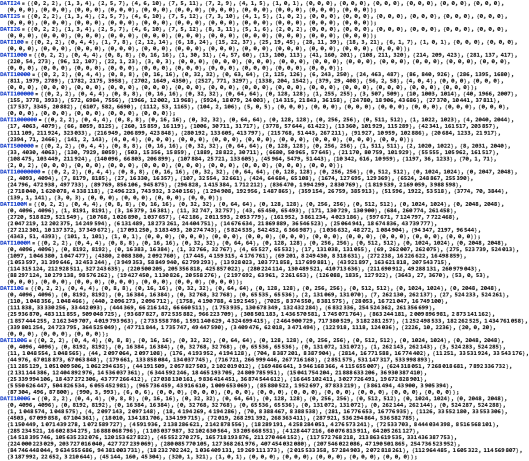
Considering the S
TC=21 system, using the script program in Appendix I we compute 30410 different {mi, vi} solutions (also see
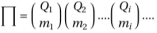
Table 1). For each of these solutions, using the approach of the statistical mechanics, we will look for the maximum number of ways in which the branching process in question can occur. We want then to compute the number of different configurations involved. To do this we resort to a combinatory tool, namely the binomial coefficient as follows:
The Π value is the number of possible configurations for any given solution. Using the whole computed solution space and the computer script in Appendix III, we plot this number sorted in descending value. We obtain the following
Figure 9 and
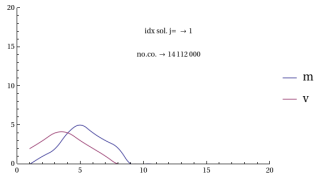
Figure 10, that shows (in linear and log scales) an initial sharp peak corresponding to the solution with the maximum no. of configurations. This max. number leads to 14112000 possible configurations. For the rest of the cases, the most part of them has an almost flat distribution (about two orders of magnitude minor); note that there is also a minimum peak, for this number, at the extreme right of the curve. Let us see in detail which solutions are 'extreme' as the number of configurations.
Figures 11 and 12 highlight these two cases for us. The data are grouped as follows: an initial lexicographic index value, then we have the list of sequences of values of the 'm' variables followed by all the 'v' variables, then we have a value that tells us at what index of the iteration the solution ends, finally we have the exact calculated value of the number of configurations.
Figure 9. The solutions for TC=21 sorted in descending order with linear scale.
Figure 10. The solutions for TC=21 sorted in descending order with log. Scalely.
Figure 11. Structure of the "most probable" solution, TC=21.
Figure 12. Structure of the "less probable" solution, TC=21.
The shapes of the two 'extreme solution' vs the configuration number are shown here under in
Figure 13 and
Figure 14 interpolating the discrete values of 'm' and 'v ' for ease of visualization.
4.2.2. The Most Probable Solution Search at High TC Values by the Application of the Fermi Statistics Method
So far, we have been looking for the maximum likelihood value of the solutions by calculating it numerically in a direct way for the available solutions of the system S when the parameter TC has low values. We now want to extend the analysis to cases with numerically unbounded TC. Computer calculation can no longer be applied because of computational limitations, so we will have to resort even more extensively to statistical methods. This study was done by the author in Ref.
. Without repeating the reasoning followed, we recall the main results hereunder. For the more general case of a system S with parameter TC >> 2 it was found that the most probable solution (i.e., with the greatest number of 'paths' configurations) is expressed by a recursive equation in the variables {m
r}
Figure 13. The maximum configuration case for a S system with TC=21.
Figure 14. The minimum configuration case for a S system with TC=21.
where we use the index 'r' to distinguish this particular solution. This recursive equation has the following aspect:
(12)
If we introduce the parameter rF= log(TC-2)/log(2), we obtain the following set of equations that represent - in recursive way - the most "probable" solution set of a diophantine S TC system with β=2. We use here the bold character and the index r to distinguish this particular solution set to the other possible solutions. The magnitude rF has a formal reference to Fermi statistics, indicating an analogy to the so-called 'Fermi level' magnitude.
(13)
From equations group (
13) some peculiar features are immediately apparent: all the variables
m, v, Q converge to zero with 'r' tending to infinity; these same variables also depend on a single parameter TC, which in turn represents the sum of the 'm' variables (according to eq. (
6)): that is, TC represents the area under the bell-shaped curve described by the m's (as will be seen below). With the S-system equations above, computer recursions can be performed by varying the TC parameters as desired, and numerical results of the most probable solution sought at high values of TC are given in Appendix IV for values of TC ranging from a few tens to 10
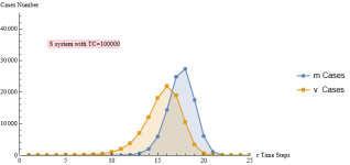
12. To show an example of curve trends with high TC values,
Table 2 calculated with TC=100000 is proposed. It should be noted that these values (such as those in Appendix IV) are rounded to the nearest unit and thus represent an approximation to the actual diophantine solution.
Table 2. r, m,v,Q values for S system with TC=100000.
r step | m | v | Q |
1 | 0 | 2 | 2 |
2 | 0 | 4 | 4 |
3 | 0 | 8 | 8 |
4 | 0 | 16 | 16 |
5 | 0 | 32 | 32 |
6 | 0 | 64 | 64 |
7 | 0 | 128 | 128 |
8 | 1 | 255 | 255 |
9 | 3 | 507 | 509 |
10 | 10 | 1003 | 1014 |
11 | 40 | 1966 | 2007 |
12 | 155 | 3778 | 3933 |
13 | 572 | 6984 | 7556 |
14 | 1966 | 12002 | 13968 |
15 | 5924 | 18079 | 24003 |
16 | 14315 | 21843 | 36158 |
17 | 24780 | 18906 | 43686 |
18 | 27370 | 10441 | 37811 |
19 | 17537 | 3345 | 20882 |
20 | 6107 | 582 | 6690 |
21 | 1112 | 53 | 1165 |
22 | 104 | 2 | 106 |
23 | 5 | 0 | 5 |
24 | 0 | 0 | 0 |
Total | 100001 | 100000 | 200002 |
We can see graphically the data shown in
Table 2 through
Figure 15:
Figure 15. The variables plot for the 'maximum likelihood' solution by recursive algorithm for S System with TC=100000.
Comparing the trend of the curves in
Figure 15 with that of the plot in
Figure 13, we notice some similarity although the TC values are very different between the two cases and the calculation algorithm used also. We also notice that the group of curves is shifted to the right on the axis that gives the number of branching steps. This is characteristic of S systems: as TC increases, the group of curves shifts to the right while still maintaining the same shape. This is shown on
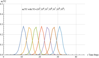
Figure 16, where plots of the 'normalized' (m/TC) data given in Appendix IV are presented with TC's ranging from 10^3 to 10^9. Below we give more details on these features.
4.2.3. Additional Properties of the Most Likely Solution
From the eq. (
13) we see that:
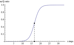
The form of this eq. leads to a Cumulative Logistic Distribution shape. This is shown in the following
Figure 17 for TC=100000, where the dashed line intercepts the curve at 0.5 level and the r axis at rF point, with rF=16.6096.
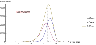
From
Figure 15, it can be seen that even if Rmax=100000-1, the set of most probable solutions will involve a number of non-null m & v variables limited to a few dozen. This is explained by the logarithmic dependence of rF with respect to TC (see eq. (
13) -first formula. We now reproduce the data in
Table 2 revised graphically as in
Figure 18 utilizing a computer interpolation algorithm to generate continuous lines (see also Ref.
). The dashed line starts at rF and intercepts -as expected- the crossing of
m and
v curves. It can be demonstrated that the peaks of the three curves conserve their relative allocation around rF value and between themselves, for any rF (and consequently TC) value.
5. Some Possible Applications
We have seen in the previous sections that the diophantine equations S, Q, U can describe general cases of branching such as:
(a) dynamics of objects or organisms’ populations
(b) a single subject choosing when faced with two or more alternatives.
Let us see in the following some examples of such situations and more.
5.1. The Volterra - Lotka eq.s Correlation
5.1.1. The Volterra - Lotka Equations
The Volterra - Lotka differential equations that describe the pattern of evolution of populations composed of prey and predators are well known. These have the form:
where N1 and N2 represent the population of prey and predators, respectively, while the others symbols are positive parameters. The model shows that in the absence of predators there would be continuous prey growth assuming unlimited availability of food. The presence of predators gives rise to the probability of prey-predator encounters via the nonlinear N1 N2 term.
5.1.2. The Correlation with the S Model
In the study of Ref.
the author proposed the differential eq. (
15) describing an S^TC system with 'v' and 'm' variables no more discrete but in continuous form, with the addition of the "logistic" not recursive condition (coming from eq.s (
13)):
and the boundary condition (by similarity with eq. (
4))
;(15)
Now if we merge the two above (
14) equations by eliminating the N1 N2 group, we get:
N1'=a1 N1-b1 a2N2/b2-b1N2'/b2;
which becomes the same expression as the previous S^TC differential equation (
15) if we impose:
In this connection we can then interpret the differential equation describing the continuous behavior of our S^TC as a special case of a Volterra - Lotka system. In such a correlation, the preys become the 'v' variables and predators are the 'm' variables. The rule would then predict that at each interval of 'v' growth, there may be a certain number of them eliminated by 'm' predators growing by the same amount. In this representation, the 'most likely' curves in
Figure 13 and
Figure 15 take on a concrete meaning: initially the 'v' curve of prey grows exponentially only to be restrained and set on a downward slope by the growth of predators in the 'm' curve. The system ends with the disappearance of the two populations since our S, Q, U systems are constrained to reach a stop condition anyway.
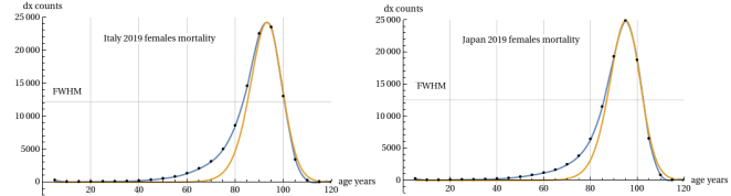
5.2. The Demographic Mortality Correlation
Looking at
Figure 18, and in particular at the m-curve representing 'fatal' events, it comes naturally to think to distribution curves of failures in real cases possibly e.g. correlated to reliability or failures accumulation models (like as recalled in Ref.
| [8] | L. A. Gavrilov and N. S. Gavrilova, "The Reliability Theory of Aging and Longevity" J. theor. Biol. (2001) 213, 527-545. |
| [9] | P. Y. Nielsen, M. K Jensen, N. Mitarai, S. Bhatt "The Gompertz Law emerges naturally from the inter-dependencies between sub-components in complex organisms"
https://doi.org/10.1038/s41598-024-51669-5 |
[8, 9]
) involving demographic effects. A significant case of application for this possible approach were demographic mortality data. National demographic agencies update their countries demographic data annually with the publication of so-called Life-Tables. These -among other things- collect mortality data of the total population (or even in regional geographic groupings etc.). The Life Tables, as far as the mortality figure is concerned, can be associated with the first two columns of our
Table 2 above. In this case the 'r' intervals will be five-year intervals of data collection, and the time range then will stretch from the first 5 years of life (r=1) to 120 years (r=24). In several recent articles (Refs.
), the author has studied this correlation between the S-system and demographic mortality, finding that a branching model and its mathematics are able to approximate well the demographic mortality curves at high ages, that is, to describe theoretically and in mathematically analytical form the "peak" mortality present in life tables. In
Figure 19 below we recall the result of Ref.
work comparing the trend of the actual demographic mortality curves for Italy and Japan with the theoretical trend of the 'm' curve of the correlated S-system. The figure shows the demographic mortality curve joining the mortality 'dx' counts for five years intervals points measured in the 2019 female Life-Tables of both countries. Underlying this real curve is the curve that would be placed with an S-system having the same peak position and with the 'm' curve scaled to coincide at the peak apex with the real curve. A value of TC=262146 and TC=201847 is found for Japan and Italy S systems. This TC parameter is the only data needed to describe the curve. You can also see that the value of Full Width at Half Maximum (FWHM on the mid-intercept line) between the real and S-curve is very similar. In practice, the S-system curves cover about 80% of the value of the real curve. The leftward asymmetry of these curves is characteristic of all real demographic mortality curves and can also be explained, within the framework of the S, Q, U theory, by the presence of additional S sub components with different and smaller TC parameters and different relative 'weights'. See on this Ref.
.
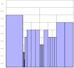
5.3. The 2d Space Partitioning
Recalling the graphical representation of S-solutions with β=2 carried out in section 3, we observe that these graphs provide a type of tiling of space in two dimensions. These partitions all have the peculiarity of showing groupings that are always rectangular in shape and look like ordered integer multiples of an 'atomic' rectangular cell. These rectangular groupings are in number of 2(TC-1) (i.e., the sum of all cases 'm' and 'v'). To see these in detail, let us consider the solution S
21 in
Figure 11 as an example. It can be seen that this solution terminates after 8 iterations. We can then assume a 'space' of 'states' structured in 8 binary steps as in
Figure 20.
The 'atomic' lattice-like rectangles to be used for our partitions buid-up will be the minimal size rectangles shown in the last step, i.e. rectangles with dimensions of 1 unit space height and 1/256-unit space width. Returning to the solution in
Figure 11 we see in the following
Figure 21 an implementation of one of the solution configurations using the graphical approach of section 3. The figure shows two groups of 'bricks' of different sizes: those in dark color and those in white.
Figure 20. Space partition mesh for 8 steps binary branching.
Figure 21. A possible partition of 2d area with 40 rectangles built over multiples of an 'atomic' unitary cell.
The former are arranged vertically while the latter are arranged horizontally. All these objects are mapped onto the mesh of
Figure 20 and thus are built-up on unit 'atomic' cell multiples. We know from section 4.2 that there are about 14112000 different possible configurations. All these configurations will have, as invariant numbers, 21 dark-colored rectangles and 19 white-colored rectangles. The two dark and white areas are always separated by a continuous segmented boundary line. Even for this line there will be 14112000 different paths. Of course, a similar representation can be made for all configurations of the 30410 solutions of the S^21 system. All these configurations are describable by the rules we have outlined and in principle can be computed and visualized as e.g. in
Figure 21. They represent possible ordered partitions of the two-dimensional plane. These partitions suggest for example patterns of fixed amount 'poly crystal-like' objects different in internal structure and forced to grow in a limited space while preserving a separation between them.
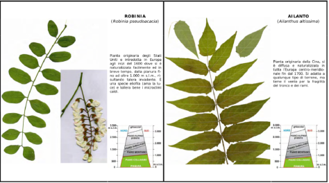
5.4. Leaves on Tree Branches and 'Stationary' Solution
If we look at
Figure 22, we see twigs with leaves from two different trees (Ref.
). They show two different types of symmetry. In the first case, the leaves develop alternately to the left and to the right but with a single bifurcation and terminate with a pair of leaves. In the second case the leaves develop with a triple branching ending in a triplet of leaves. If we now associate to the birth of the leaflet the event of type 'm' while to the body of the branch (which continues without 'collapsing' into a leaf) we associate the event of type 'v', we can see the two cases as a 'stationary' solution of two S-systems, the first with β =2 and the second with β =3.
The stationary solutions for the two cases will be:
first case: {m sol.} ={..,1,1,1,1,2}; {v sol.} = {...,1,1,1,1,0}; β=2, with alternate left-right configuration for the m=1 event
second case: {m sol.} = {..,2,2,2,2,3}; {v sol.} = {...,1,1,1,1,0}; β=3;
We can now consider a branching process in which initially the cells that multiply are only of type 'v' (thus increasing in exponential number without the 'm' (leaf) component). This branching process ends at a certain iteration step and at the terminal of each ‘v’ branch thus produced, we imagine grafting branches with leaves identical in structure to those described in
Figure 22. In this model, we obtain a tree structure similar to the real trees of the two types described above, with the inner branches devoid of leaves that will instead be found in the final outer branches crown. In any case all the sequences are terminated with leaves, thus leading to a more general S system built up with the sum of ‘small’ steady state sub-solutions. We can therefore say that -for this type of real trees- the system S is applicable and the solution chosen in nature -of the many possible ones- is the one we call 'steady state'.
6. Summary and Conclusions
In the previous sections we introduced some mathematical definitions and properties for three classes of diophantine equations, called S, Q, U. They quantitatively describe branching processes in which objects (or situations) can multiply in successive iterations. The multiplicative factor β considered in the study is equal to two. Theorems statements, systems properties and numerical examples are also given in Appendices. Two additional elements also characterize these systems S, Q, U:
- the presence of an independent random integer variable acting in subtraction to the generated objects (the m cases)
-the mathematical constraint of the limiting number of cases generated (or the maximum number of iterations), which implies reaching the end of the branching process life cycle. These constraints are numerically based on the TC ("Total Cases") parameter.
The S, Q, U equations always admit solutions for the independent random integer variables. A graphical representation of these solutions has been provided to facilitate understanding of the structure itself. Some of these solutions are interesting for the purpose of finding practical applications. Two of these solutions were studied in the case of S systems and β=2, to find stationary solutions or the 'most probable' solution. For this last purpose, the methods of Fermi statistics were used. The 'most probable' solution, even for very high values of the TC parameter, converges quite rapidly after relatively few iterative steps. The study mentioned some possible applications of the S, Q, U systems in real cases. In this connection and in other research papers, the author developed detailed research on demographic mortality patterns describable by the S system equations and proposing a conjecture about the trend of demographic mortality as longevity increases. See on these aspects the studies in Ref.
. The main purpose of the study proposed here is the realization of a mathematic infrastructure to describe constrained branching cases. The proposed system of equations allows the identification of meaningful solutions of the possible evolutions of the systems themselves. The study focuses particularly on the case of binary branching for systems S. In the future, it might be interesting to analyze the extension of these processes to cases with β>2 and/or with β that can change during iterations as an additional integer variable. Another interesting aspect of S, Q, and U systems is that they include solutions that show regularity and repetitive patterns (such as stationary solutions and the most probable solution that maintains a form invariance even when the TC parameter varies). This stationarity of binary growth is present, for example, in the growth of microbial masses Ref.
. The characteristic of S, Q, U systems to show regular solutions - among the many possible ones - in the face of constraints, can also fall within a broader class of studies related to 'emerging' phenomena where apparently complex structures composed of many 'atomic' elements can give rise to regular forms and structures on a larger and macroscopic scale. Ref.
| [16] | E. Nocerino "Emergent properties and the multiscale characterization challenge in condensed matter, from crystals to complex materials: a Review", arXiv:2503.20266v1 [cond-mat.mtrl-sci] 26 Mar 2025 |
| [17] | R. Solé, C.P. Kempes, B. Corominas-Murtra, M. De Domenico, A. Kolchinsky, M. Lachmann, E. Libby, S. Saavedra, E. Smith, D. Wolpert "Fundamental Constraints to the Logic of Living Systems", https://doi.org/10.20944/preprints202406.0891.v1 |
[16, 17]
. The case of the correlation of S solutions with the botanical structures mentioned in subsection 5.4 may ultimately be explored in a future study to verify whether S, Q, U systems can describe classes of tree configurations (such as those predicted experimentally in the work of Ref.
| [18] | F. Hallé, R.A.A. Oldeman, P.B. Tomlinson " Tropical trees and forests " Springer-Verlag, 1978. |
[18]
) or whether, by applying Lindenmayer's iterative methods, it will be possible to represent solutions of S, Q, U systems in the form of L-Systems applied to tree structures. (Ref.
| [19] | P. Prisinkiewickz, A. Lindenmayer "The algorithmic beauty of plants", Springer-Verlag, 1990. |
[19]
).
Abbreviations
ArbO | Arbitrary Oscillator |
FWHM | Full Width at Half Maximum |
Author Contributions
Giuseppe Alberti is the sole author. The author read and approved the final manuscript.
Funding
This work is not supported by any external funding.
Data Availability Statement
The data supporting the outcome of this research work has been referred in this manuscript.
Conflicts of Interest
The author declares no conflicts of interest.
Appendix
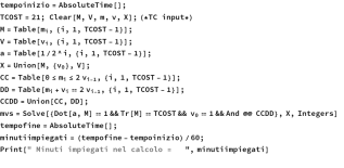
Appendix I: Solutions Scripts
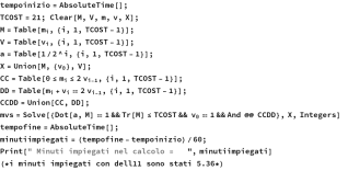
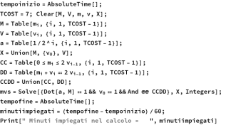
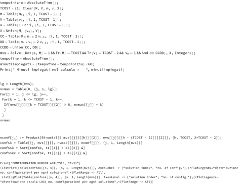
We give in the following the computer scripts used to calculate the S, Q, U solutions, complete in the variables 'm 'and 'v' and for the case TC=21. The script is designed in compact form such that it can be used with an arbitrary input TC value and consequently any imax (=TC-1) number of variables. The machine time of the calculation for the TC=21 case is about 3 minutes with a standard notebook. The script runs under a well-known commercial mathematical calculation application. The script looks for all possible solutions of the two equations of the system S with the parameter TC fixed as input. As the value of TC increases, soon the limit of computational overhead is reached for values just above about 25 for the S and Q cases.
The script below applies to the case of System S, TC=21:
The next script applies to the case of System Q, TC=21
Finally, the script for the case of System U, TC=7:
Appendix II: Some Theorems
In the following we provide some theorems statements. These theorems statements are referred to the case β=2. We use the S' system apex notation meaning a S system with TC' parameter, then a S'' system means a system with TC'' parameters etc. At the same time the expression S+1 means a system with TC+1 parameter or an expression S'+S'' leads to a TC'+TC'' parameter system. In general, we can also use the notation with evident meaning. In general, we use the STC, QTC, UTC notation with evident meaning. In addition, we use the symbol { XTC } to mean the set of all solutions of XTC.
Moreover, we use the notation:
to address some conditions on XTC variables with X=S,Q,U.
T0 - The "total" Theorem
T1 - The "one" Theorem
If {mi} is a solution of a S system, then the list {1, {mi}} is a solution of the S+1 system.
This implies that all the solutions of a S system are solutions of a S+1 system if prepended by "1".
T2 - The "zero" Theorem
If {mi'} is a solution of a S' system, and {mi''} is a solution of S'' system, then the list {0, {mi'+mi''} } is a solution of a S'''= S' +S'' system. This implies that all the solutions of a S''' system that have m1''' = 0, can be expressed by an index ordered sum of two solutions terms mi'+mi'' belonging to subsystems S' and S'' where S'''= S'+S''.
T2 - C1 Corollary
If m1=0, then also mimax=0
T3 - The "alpha" Theorem
Given iα<= imax, at least a mi of {mi} with the index 1≤ i ≤ iα must be not null being: iα= Int(log2TC)
T4 - The "sum" Theorem
The solutions of a QTC system are given by the union set of all solutions of STC,STC-1,.., S2
T5 - The "inclusion" theorem
The solutions of a QTC system are included in the set of all the solutions of UTC
T6 – Theorem
This theorem links the solution set of a U^TC system with a subset of solutions coming from a higher "rank" Q system.
This theorem is a consequence of the general condition addressed above.
This theorem is depicted by the formula:
NOTE: As a quick check for the above theorems, the reader can easily see that, as in section 2.2, example No.3, there are two solutions which begin with "1". These are obtained directly by the two solutions of S
4 prepended by "1". In turn, the "0" solution is given by summing the single solutions of S
2 and S
3 subsystems. For the T3 theorem the reader can e.g. check with the plenty of possible solutions listed in Ref.
| [7] | G. Alberti, Web site managed by the author and devoted to diophantine STC equation systems. https://squ-systems.eu |
[7]
for the case TC=14. By virtue of T4 theorem, a generic Q system can be built up by knowing the solutions of subsystems S with smaller or equal TC parameters. However, lacking a numeric formula to find solutions number and values for a S system, this also limits the general description of Q systems.
Appendix III: Configurations Script
In the following we give the script used for calculating the number of configurations for all solutions of a binary system S, β=2. The script also provides for the ordering of the solutions found in the three ways: 1) lexicographic, 2) no. of configurations, 3) nvmax index (last step i with vi non-zero). It is also given the plot command for a graphical view of the results. The following script example refers to TC=21, but the script accepts any value of TC as input.
Appendix IV: Solutions Data
Solutions (most probable solutions rounded to integer value) for a recursive S system with TC ranging from 24 to 10^12; format: DATI<TC>={{mr,vr,Qr}}:
References
| [1] |
M. Kimmel, D.E. Axelrod. "Branching processes in Biology", Springer, 2002.
|
| [2] |
S. Méléard, "Modèles aléatoires en Ecologie et Evolution", Springer, 2016.
|
| [3] |
N. Bacaer, "Histoires des mathematiques et de populations", ed. Cassini, Paris, 2008.
|
| [4] |
J. Kaandorp, "Fractal modelling growth and form in biology", Springer-Verlag, 1994.
|
| [5] |
A. Vulpiani, " Determinismo e caos", Carocci, 2004.
|
| [6] |
G. Alberti "Fermi statistics method applied to model macroscopic demographic data"
https://arXiv.org/abs/2205.12989
|
| [7] |
G. Alberti, Web site managed by the author and devoted to diophantine STC equation systems.
https://squ-systems.eu</i>
|
| [8] |
L. A. Gavrilov and N. S. Gavrilova, "The Reliability Theory of Aging and Longevity" J. theor. Biol. (2001) 213, 527-545.
|
| [9] |
P. Y. Nielsen, M. K Jensen, N. Mitarai, S. Bhatt "The Gompertz Law emerges naturally from the inter-dependencies between sub-components in complex organisms"
https://doi.org/10.1038/s41598-024-51669-5
|
| [10] |
G. Alberti "A conjecture on demographic mortality at high ages."
https://arxiv.org/abs/2307.10279
|
| [11] |
G. Alberti "More on the mortality conjecture: the components of demographic mortality"
https://doi.org/10.13140/rg.2.2.14304.46086
|
| [12] |
G. Alberti "On two asymptotic limits for demographic mortality Life Tables data"
https://doi.org/10.13140/rg.2.2.27428.86405
|
| [13] |
G. C.Perosino, P. Zaccara "ATLANTE DELLE FOGLIE E DELLE 50 SPECIE ARBOREE PIÙ DIFFUSE NELL'ITALIA SETTENTRIONALE CONTINENTALE"-CREST
HYPERLINK "
http://www.crestsnc.it/divulgazione/media/chiave.pdf"
http://www.crestsnc.it/divulgazione/media/chiave.pdf
|
| [14] |
J. W. Fink, M. Manhart "How do microbes grow in nature? The role of population dynamics in microbial ecology and evolution",
https://www.sciencedirect.com/journal/current-opinion-in-systems-biology
Volume 36, December 2023, 100470
|
| [15] |
H. Laurie "A class of models that support a maximum entropy principle for age structure",
https://doi.org/10.20944/preprints202305.2151.v1
|
| [16] |
E. Nocerino "Emergent properties and the multiscale characterization challenge in condensed matter, from crystals to complex materials: a Review", arXiv:2503.20266v1 [cond-mat.mtrl-sci] 26 Mar 2025
|
| [17] |
R. Solé, C.P. Kempes, B. Corominas-Murtra, M. De Domenico, A. Kolchinsky, M. Lachmann, E. Libby, S. Saavedra, E. Smith, D. Wolpert "Fundamental Constraints to the Logic of Living Systems",
https://doi.org/10.20944/preprints202406.0891.v1
|
| [18] |
F. Hallé, R.A.A. Oldeman, P.B. Tomlinson " Tropical trees and forests " Springer-Verlag, 1978.
|
| [19] |
P. Prisinkiewickz, A. Lindenmayer "The algorithmic beauty of plants", Springer-Verlag, 1990.
|
Cite This Article
-
ACS Style
Alberti, G. Properties of a System of Diophantine Equations with Implications for Real-World Constrained Branching Processes. Sci. J. Appl. Math. Stat. 2025, 13(5), 111-127. doi: 10.11648/j.sjams.20251305.12
 Copy
|
Copy
|
 Download
AMA Style
Alberti G. Properties of a System of Diophantine Equations with Implications for Real-World Constrained Branching Processes. Sci J Appl Math Stat. 2025;13(5):111-127. doi: 10.11648/j.sjams.20251305.12
Copy
|
Download
-
@article{10.11648/j.sjams.20251305.12,
  author = {Giuseppe Alberti},
  title = {Properties of a System of Diophantine Equations with Implications for Real-World Constrained Branching Processes},
  journal = {Science Journal of Applied Mathematics and Statistics},
  volume = {13},
  number = {5},
  pages = {111-127},
  doi = {10.11648/j.sjams.20251305.12},
  url = {https://doi.org/10.11648/j.sjams.20251305.12},
  eprint = {https://article.sciencepublishinggroup.com/pdf/10.11648.j.sjams.20251305.12},
  abstract = {We consider an iterative branching process in which an abstract object can subdivide into other objects. The multiplication process may be varied by the occurrence of random "fatal" events in which some of the subsequent objects or states may fail. The process is also constrained to terminate upon reaching a given number of events or alternatively upon reaching a fixed number of iteration steps. A system of diophantine integer-variable equations capable of describing the aforementioned process is proposed. These equations can be applied prospectively to many branching phenomena of physical, biological and demographic nature. The equations, which we call systems of equations S, Q, U can be reformulated into three main classes based on the behavior of the sum of variables with respect to a fixed principal numerical parameter (TC= 'Total Cases'). These systems always admit solutions and these are sought for the three classes. The mathematical properties of the three systems are presented both analytically and graphically, and the software script for calculating numerical solutions is attached. In the case of high TC values, where direct calculation is not possible, special solutions are also sought for the steady state case and the "most probable" case, the latter using statistical mechanics methods. Solutions examples are given for a wide range of TC parameters. We also refer to real-world examples of applications ranging from prey/predator population dynamics to population mortality modeling and 2d lattice space tiling and also tree leaves branching alternatives. The main purpose of the study here proposed is to implement a mathematical frame that can provide tools to be used in the study of real-world applications.},
 year = {2025}
}
Copy
|
Download
-
TY  - JOUR
T1  - Properties of a System of Diophantine Equations with Implications for Real-World Constrained Branching Processes
AU  - Giuseppe Alberti
Y1  - 2025/12/27
PY  - 2025
N1  - https://doi.org/10.11648/j.sjams.20251305.12
DO  - 10.11648/j.sjams.20251305.12
T2  - Science Journal of Applied Mathematics and Statistics
JF  - Science Journal of Applied Mathematics and Statistics
JO  - Science Journal of Applied Mathematics and Statistics
SP  - 111
EP  - 127
PB  - Science Publishing Group
SN  - 2376-9513
UR  - https://doi.org/10.11648/j.sjams.20251305.12
AB  - We consider an iterative branching process in which an abstract object can subdivide into other objects. The multiplication process may be varied by the occurrence of random "fatal" events in which some of the subsequent objects or states may fail. The process is also constrained to terminate upon reaching a given number of events or alternatively upon reaching a fixed number of iteration steps. A system of diophantine integer-variable equations capable of describing the aforementioned process is proposed. These equations can be applied prospectively to many branching phenomena of physical, biological and demographic nature. The equations, which we call systems of equations S, Q, U can be reformulated into three main classes based on the behavior of the sum of variables with respect to a fixed principal numerical parameter (TC= 'Total Cases'). These systems always admit solutions and these are sought for the three classes. The mathematical properties of the three systems are presented both analytically and graphically, and the software script for calculating numerical solutions is attached. In the case of high TC values, where direct calculation is not possible, special solutions are also sought for the steady state case and the "most probable" case, the latter using statistical mechanics methods. Solutions examples are given for a wide range of TC parameters. We also refer to real-world examples of applications ranging from prey/predator population dynamics to population mortality modeling and 2d lattice space tiling and also tree leaves branching alternatives. The main purpose of the study here proposed is to implement a mathematical frame that can provide tools to be used in the study of real-world applications.
VL  - 13
IS  - 5
ER  -
Copy
|
Download